

Capabilities · Process CFD and mixing
A flow simulation earns trust only beside a measurement
Computational fluid dynamics (CFD) solves the equations of fluid motion inside a vessel to predict velocity, shear, mixing and heat transfer where no probe can reach. In published work on one laboratory vessel, four simulation set-ups predicted its power draw with errors from −4% to +12%. EUTECNIQ proposes to use CFD with qualified partners and to test every prediction against measured power, blend time or velocity.
Proposed capabilityEUTECNIQ holds no CFD software licenses or computing hardware, has run no simulations and has measured no vessels. Figures re-plot values reported in open-access papers; the calculator is an educational model, not a design.
Power number of one 2.8 L vessel: four CFD set-ups against the torque measurement
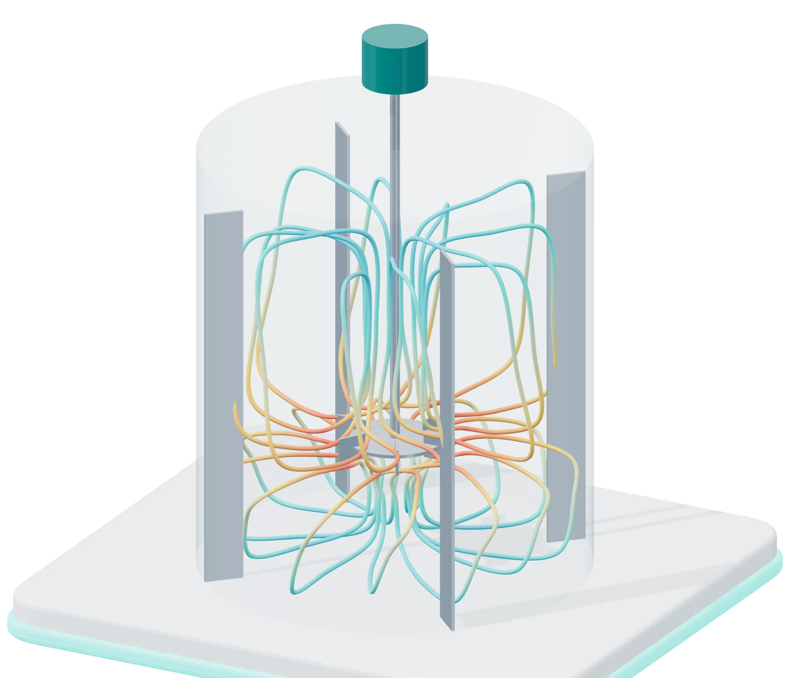
- 1 Radial jet from the impeller
- 2 Upper circulation loop
- 3 Lower circulation loop
- 4 Baffles stop the liquid swirling
The flow pattern a six-blade disk turbine produces in a baffled tank: a radial jet and two circulation loops. Color shows relative speed, fastest at the impeller tip. An illustration, not a simulation result.
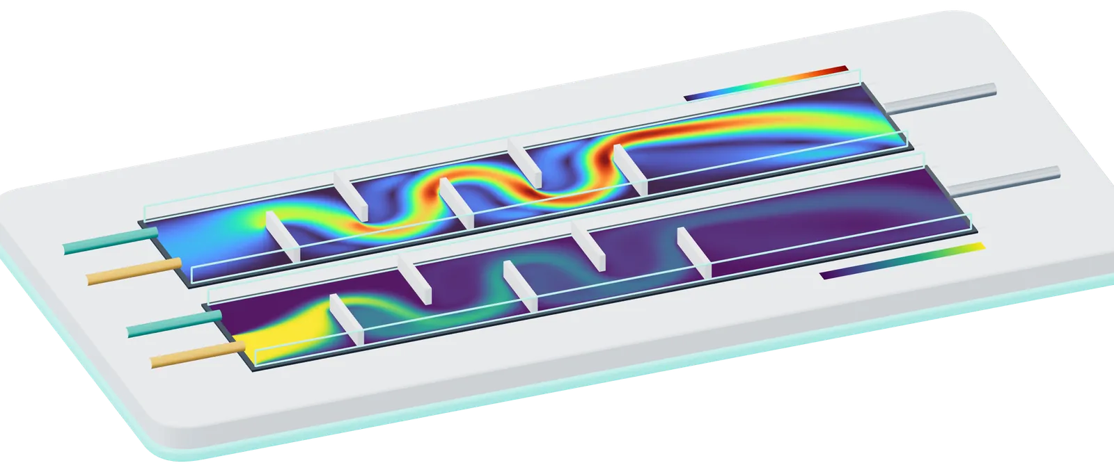
- 1 Feed A (amber)
- 2 Feed B (teal)
- 3 Baffles turn the flow; jets and eddies form behind each one
- 4 Speed of the flow, relative to the mean inlet speed
- 5 Fraction of feed A: the two streams blend baffle by baffle
- 6 Outlet
Color scales: speed from 0 to 6.5 times the mean inlet speed; fraction of feed A from 0 to 1. Computed by EUTECNIQ for this page: two-dimensional lattice Boltzmann method (D2Q9, single-relaxation-time BGK; Zou–He velocity inlet and pressure outlet), 560 × 96 lattice, Reynolds number 52 based on channel width and mean inlet speed, a snapshot after 110,000 time steps; density stayed within 1% below to 5% above its outlet value, so compressibility error is small. Feed A’s fraction is a passive scalar carried by the computed flow with a first-order upwind scheme, whose numerical diffusion overstates mixing. Illustrative geometry; a 2D laminar calculation, not validated against experiment and not a design of any EUTECNIQ equipment.
01 · The problem it solves
Correlations give a vessel's averages; CFD shows where mixing, shear and heating fall short
A power curve and a blend-time correlation describe a whole tank with one number each. Extraction, emulsification and drying often fail locally, in a stagnant corner, a high-shear zone at the impeller tip or a hot spot on a dryer wall. CFD estimates those local fields, but only within limits that have to be checked.
- Flow field: velocity everywhere in the vessel, including slow zones a sample port would miss
- Mixing: how a tracer spreads and how long the batch takes to become uniform
- Shear and energy dissipation: where droplets break or fragile material is damaged
- Heat transfer: wall and coil temperatures and local heating rates
- Residence time: how long fluid parcels stay in a continuous device or a dryer chamber
- Whether the answer is right, which needs a measurement on the same geometry
- Errors from the turbulence model, which approximates eddies it does not resolve
- Errors from the mesh, until a refinement study shows the result no longer moves
- The behavior of a slurry whose viscosity has not been measured
- Droplet breakage, cavitation or particle sticking where sub-models are still immature
Next: see the equations and the six steps every credible simulation follows.
02 · The mechanism
Every simulation solves the same conservation laws; the modeling choices around them set its accuracy
The governing set, which NASA's reference calls the Navier–Stokes equations, is a continuity equation (mass), three momentum equations and an energy equation. It is too difficult to solve analytically, so software solves approximations of them numerically on a mesh, the vessel volume divided into small cells.
RANS (Reynolds-averaged Navier–Stokes) solves for the time-averaged flow and represents all turbulent eddies with a model such as k–ε or k–ω, which carry the turbulent kinetic energy and its dissipation rate. LES (large-eddy simulation) resolves the large eddies in time and models only the smallest. LES needs far finer meshes and longer runs.
A steady multiple reference frame (MRF) treats the zone around the impeller as rotating and the rest as still, which is cheap. A sliding mesh or a transient method moves the impeller and captures the unsteady flow. The size of the rotating zone itself changes the answer.
Water needs a density and a viscosity. A botanical slurry or puree usually needs a viscosity that falls with shear rate (a power law, or Herschel–Bulkley with a yield stress), fitted to a measured flow curve. Without that curve the simulation borrows numbers from another material.
The six steps of a simulation that can be audited Educational schematic
- GeometryVessel, impeller, baffles, coils and nozzles as built, with the liquid level of the batch.
- MeshCells fine enough near blades and walls; a coarse, a medium and a fine version for the refinement study.
- ModelTurbulence closure, impeller treatment, measured rheology, heat and phase sub-models.
- SolveIterate until residuals and the monitored quantities (torque, velocity at a point) stop changing.
- VerifyCompare the three meshes; report the apparent order of convergence and the grid convergence index.
- ValidateCompare with a measurement on the same geometry: torque, blend time, or velocities by PIV or LDA. If it fails, return to the mesh or the model.
Equations: NASA Glenn Research Center, Navier–Stokes Equations (updated May 13, 2021). Verification: Celik IB et al., J Fluids Eng 2008;130:078001 (three significantly different grids; refinement factor preferably above 1.3). MRF and rotating-zone size: Kuschel et al. 2021. PIV: particle image velocimetry; LDA: laser Doppler anemometry.
Next: see how much the modeling choices moved one published result.
03 · Validation evidence
The rotating-zone layout alone moved one vessel's predicted power number by 16%
Kuschel and colleagues measured the torque of a 2.8 L laboratory vessel with two Rushton turbines in water and simulated it with steady RANS and with a transient lattice-Boltzmann LES. Changing only the layout of the rotating zone moved the RANS power number from 7.2 to 8.4, a spread of 16% of the measured 7.5; the authors found zone size as influential as mesh size.
- Steady RANS: cell counts from 100,000 to 700,000 tested; about 350,000 polyhedral cells were fine enough for the power number, which settled near 8.1
- Lattice-Boltzmann LES: 1.7 to 379 million lattice points tested; velocity stopped changing at 27 million, with the power number at 7.5 ± 0.5
- Highest velocity at 250 rpm, in under 10⁻³% of the volume: 0.47 m/s simulated against 0.51–0.58 m/s measured by particle tracking
- A mesh that is good enough for power draw can be too coarse for shear or velocity peaks
- The refinement study has to be repeated for the quantity the decision depends on
- Rotating-zone size belongs in the study, alongside the mesh
| Method | Power number | Difference from measured 7.5 |
|---|---|---|
| Torque measurement | 7.5 | reference |
| Steady RANS, realizable k–ε, mesh study (about 350,000 cells) | ≈ 8.1 | +8% |
| Steady RANS, two separate rotating zones (preferred by the authors) | 8.4 ± 0.2 | +12% |
| Steady RANS, one combined rotating zone | 7.2 ± 0.2 | −4% |
| Transient lattice-Boltzmann LES, Smagorinsky closure | 7.5 ± 0.5 | 0% |
Published evidence Kuschel M, Fitschen J, Hoffmann M, von Kameke A, Schlüter M, Wucherpfennig T. Processes 2021;9(6):950, doi:10.3390/pr9060950. RANS in ANSYS Fluent 19.0; LES in M-Star CFD 2.10.57. Differences computed here from the reported values.
04 · Critical parameters: rheology
In a published shear-thinning case, adding a turbulence model made the velocity prediction worse
Milled herb in solvent, purees and gum solutions thin as they are sheared, so their viscosity, and with it the Reynolds number, changes from the impeller tip to the wall. Story and Jaworski simulated a 0.2% Carbopol solution (τ = 15.9·γ̇0.34 Pa) and checked the results against torque and laser Doppler measurements.
Power number against Reynolds number, 0.2% Carbopol: measured and CFD
Deviation of CFD velocities from laser Doppler data, by turbulence treatment
Data tables for both figures
| Re | Po measured | Po CFD | Deviation, % |
|---|---|---|---|
| 9 | 12.61 | 13.08 | 3.7 |
| 27 | 4.36 | 4.50 | 3.2 |
| 54 | 2.54 | 2.60 | 2.4 |
| 87 | 2.21 | 2.28 | 3.2 |
| 126 | 1.95 | 1.98 | 1.5 |
| 170 | 1.84 | 1.80 | 2.2 |
| Set-up | Axial | Radial | Tangential |
|---|---|---|---|
| Laminar | 2.1 | 2.5 | 3.6 |
| Low-Re k–ε | 2.9 | 3.9 | 7.3 |
| Low-Re k–ω | 2.5 | 3.7 | 4.9 |
At Re between 9 and 170 the flow was laminar to early transitional, and adding a turbulence model doubled the tangential error with k–ε. The model has to match the regime, and the regime depends on a measured viscosity.
Metzner–Otto method, elastic effects and an unmeasured puree
The Metzner–Otto method assigns a shear-thinning fluid one average shear rate, γ̇ = ksN, from which an apparent viscosity and a Reynolds number follow. The constant ks depends on the impeller and is measured: for the Prochem Maxflo T, Story and Jaworski's CFD gave volume-mean values from 19 to 27 as Re rose from 9 to 170, against 20 from power measurements in the literature they cite; a later study of the same impeller type assumed 11 (Story A, Jaworski Z, Simmons MJ, Nowak E. Chem Zvesti 2018;72:593–602, doi:10.1007/s11696-017-0307-4).
The authors note that Carbopol may be slightly elastic, which a purely viscous model ignores. In a CFD study of a screw press for cassava leaves, no rheological data for the leaf puree existed, so data for mint puree were used, and the authors recommend measuring the puree's properties (Latif et al. 2020).
05 · Interactive model: scale-up by dimensionless numbers
From 5 L to 2,000 L, holding power per volume slows blending about fourfold
Three hypothetical, geometrically similar vessels share liquid height equal to tank diameter and an impeller one third of that diameter. Choose the impeller, the fluid, the laboratory speed and the scale-up rule; the table recomputes the Reynolds number, power, power per volume, tip speed and blend time at each scale.
Interactive calculator Change the inputs and the result updates. An educational simulation with stated inputs.
P = Po·ρN³d⁵
Nθ₉₅ = 5.2·Po−1/3(T/d)²
P/V rule: N₂ = N₁(T₁/T₂)2/3
Tip-speed rule: N₂ = N₁(T₁/T₂)
Turbulent at every scale: the constant power number and the blend-time correlation apply.
| Quantity | Laboratory5 L | Pilot100 L | Production2,000 L |
|---|---|---|---|
| Tank diameter T, m | 0.185 | 0.503 | 1.366 |
| Impeller diameter d, m | 0.062 | 0.168 | 0.455 |
| Speed N, rpm | 300 | 154 | 79 |
| Tip speed πNd, m/s | 0.97 | 1.35 | 1.89 |
| Viscosity μ, mPa·s | 1.00 | 1.00 | 1.00 |
| Reynolds number Re | 19,000 | 72,000 | 273,000 |
| Power P, W | 0.561 | 11.2 | 225 |
| Power per volume, W/m³ | 112 | 112 | 112 |
| Blend time θ₉₅, s | 5.5 | 10.7 | 20.7 |
n/a: Re below 10⁴, where the power number varies with Re and the blend-time correlation does not hold; power must come from the impeller's measured power curve. Power numbers: Rushton 5.0 is a design value inside the 3.6–5.9 range reported for baffled vessels (Kaiser et al. 2018); pitched-blade values measured at d/T = 1/3 (Fořt and Jirout 2011). Blend time: Grenville and Nienow correlation as given by Fořt and Jirout 2011 (constant 5.2 ± 10%, H/T = 1, turbulent). Kaiser SC, Werner S, Jossen V, Blaschczok K, Eibl D. J Vis Exp 2018;(135):56078, doi:10.3791/56078. Fořt I, Jirout T. Chem Process Eng 2011;32(4):311–319, doi:10.2478/v10176-011-0025-3.
Method, assumptions and limits
- What it calculates
- For three geometrically similar vessels, the impeller speed set by the chosen rule from the laboratory speed, then tip speed, viscosity, Reynolds number and, where Re ≥ 10⁴, power, power per volume and the time to 95% homogeneity.
- Equations
- Vessel V = πT³/4 (liquid height H = T), d = T/3; P/V rule N₂ = N₁(T₁/T₂)2/3, because P/V ∝ N³d²; tip-speed rule N₂ = N₁T₁/T₂; Re = ρNd²/μ; P = PoρN³d⁵; θ₉₅ = 5.2(T/d)²/(NPo1/3). For Carbopol, μ = K(ksN)n−1 (Metzner–Otto).
- Variables and units
- Volumes 5, 100 and 2,000 L; N in rpm (÷ 60 to s⁻¹); T, d in m; ρ in kg/m³; μ in Pa·s (shown in mPa·s); P in W; P/V in W/m³; θ₉₅ in s.
- Assumptions
- Fully baffled, flat-bottomed, single impeller, geometric similarity, single liquid phase. Water at 20 °C from the IAPWS formulations via CoolProp. Carbopol: K = 15.9 Pa·sⁿ and n = 0.34 measured at 20.5 °C by Story and Jaworski 2017; density assumed 1,000 kg/m³; ks is an input because it depends on the impeller.
- Valid range
- Power and blend time only for Re ≥ 10⁴ (Fořt and Jirout 2011; Kaiser et al. 2018 found the Rushton power number constant above this). Below it the cells read n/a and a notice appears.
- What it does not establish
- Solids suspension, gas dispersion, heat transfer, local shear peaks, or the real power number of a vessel, which depends on clearance, baffles and blade thickness and is measured by torque. No vessel or result here is EUTECNIQ's.
- Verification
- An independent reference calculation (numpy, CoolProp for water) recomputes every displayed value for eight input sets.
Under constant power per volume the 2,000 L vessel turns slower, so its turbulent blend time is about 3.8 times the laboratory's; under constant tip speed, power per volume falls about sevenfold. With the Carbopol option, Re stays far below 10⁴ at every scale and the turbulent rules no longer apply.
Next: more scale-up rules, including constant Reynolds number and constant blend time, are on the scale-up and tech-transfer page.
06 · Applications in botanical processing
Published studies show where CFD helped and where a simpler model predicted better
Three equipment classes in botanical and formulation work have open-access CFD studies with measurements. Each shows a different limit.
Latif and colleagues simulated cassava-leaf puree in a screw press as a Herschel–Bulkley fluid. The simulated press-head temperature, 40.6 °C, was close to the measured 44.7 °C. Juice yield could not be simulated because the rheology of the juice was unknown.
Published evidenceThaker and Ranade found that their earlier CFD–population-balance models could not capture how cavitation shaped droplet sizes in a vortex-based device. A 2026 follow-up notes that full CFD with population balances remains limited by complexity, cost and uncertain parameters.
Published evidenceFor a laboratory spray dryer, Milanesi and colleagues found that a thermodynamic balance tuned by machine learning predicted outlet temperature with a mean absolute error of 1.74 K. Their untuned CFD model erred by 10.43 K in atomizing runs.
Published evidence| Runs and model | RMSE, K | R² | Mean absolute error, K |
|---|---|---|---|
| Air only, thermodynamic balance | 4.04 | 0.99 | 3.34 |
| Air only, CFD | 7.21 | 0.99 | 6.32 |
| Atomizing, thermodynamic balance | 2.15 | 0.99 | 1.74 |
| Atomizing, CFD | 14.91 | 0.69 | 10.43 |
Latif S, Romuli S, Barati Z, Müller J. Food Sci Nutr 2020;8:3089–3098, doi:10.1002/fsn3.1517. Thaker AH, Ranade VV. Ind Eng Chem Res 2023;62:18837–18851, doi:10.1021/acs.iecr.2c03714. Pandey DK, Kumar R, Ranade VV. ACS Omega 2026;11:16248–16258, doi:10.1021/acsomega.5c11513. Milanesi A et al. Pharmaceutics 2022;14:296, doi:10.3390/pharmaceutics14020296. The authors note that the thermodynamic model was fitted to the data and the CFD model was not.
Next: drying and emulsion physics are covered on the drying and particle engineering and emulsions and colloids pages.
07 · How EUTECNIQ would decide
A correlation comes first, CFD answers local questions, and a measurement settles both
CFD costs engineering time and computing, and its error is unknown until it is tested. EUTECNIQ proposes to choose the cheapest tool that can answer the question, then name the measurement that would prove the answer.
| Question | First tool | When CFD is justified | Measurement that decides |
|---|---|---|---|
| Power draw and blend time of a standard, baffled, turbulent vessel | Power number and blend-time correlation | Non-standard impeller, baffles, coils or liquid level | Torque; tracer blend time |
| Dead zones, shear peaks or caverns | CFD | Whenever the answer depends on location | PIV, LDA or tracer visualization in a laboratory vessel |
| Mixing of a botanical slurry or puree | Measured flow curve; Metzner–Otto estimate of Re | Re in the laminar or transitional range; cavern formation | Rheometry of the actual material; torque |
| Spray-dryer outlet temperature | Heat and mass balance | Wall deposition, residence time or chamber redesign | Outlet temperature and humidity; deposit mapping |
| Droplet size from a homogenizer or cavitation device | Measured size distribution against passes and pressure drop | Only with a breakage model validated for that device | Laser diffraction of the emulsion |
Proposed capability EUTECNIQ's proposed decision rule, drawn from the studies cited on this page; it is not a published standard.
Next: energy questions often belong to a balance first; see exergy analysis and pinch analysis.
08 · Proposed deliverables
EUTECNIQ would commission CFD from partners and report it beside the measurement that tests it
A simulation report without its mesh study and its validation measurement cannot support a scale-up decision. EUTECNIQ proposes to deliver both together.
- State the decision and the acceptance criterion before any run
- Specify the laboratory measurement: torque, blend time or velocity
- Require a three-mesh refinement study and the rotating-zone check
- Combine results with the mass and energy balances
- Run licensed commercial or open-source CFD software on their hardware
- Provide PIV or LDA facilities and torque-instrumented vessels
- Measure the rheology of the actual slurry
- Software licenses, computing hardware or measurement rigs
- Simulations, validated models or vessel data
- That the calculator on this page is a design
Discuss a mixing or scale-up question
Describe the vessel, the material and the decision at stake; EUTECNIQ would respond with a proposed modeling and measurement plan and its limits.
Health information notice. These statements have not been evaluated by the Food and Drug Administration. Nothing on this site is intended to diagnose, treat, cure or prevent any disease, and nothing here is medical advice.
Read the full notice
The information is for general education only. It does not replace advice, diagnosis or treatment from a qualified health professional, or any medication a clinician has prescribed. Do not start, stop or change any medicine, supplement or herbal product because of something you read here. Talk to your doctor or pharmacist first, especially if you are pregnant or breastfeeding, have a medical condition, take any medicines, are preparing for surgery, or are caring for a child. Research findings, traditional uses and safety data are reported as their sources state them; they are not recommendations or claims about any product. If you think you may have a medical emergency, call your doctor or 911 at once.
EUTECNIQ Sciences sells no supplements or health products today and receives nothing from any product or ingredient mentioned on this site; any commercial interest it later has in an ingredient will be stated on that ingredient’s page.