

Computational research · Figure atlas
Figure atlas
All 60 figures at full resolution. Select an image to enlarge it; each figure links to its vector file and its data.
Labeled figuresThe colored label on each figure gives its evidence status; method, sources and limitations are listed under it.
FIG 001–007
Molecular structure
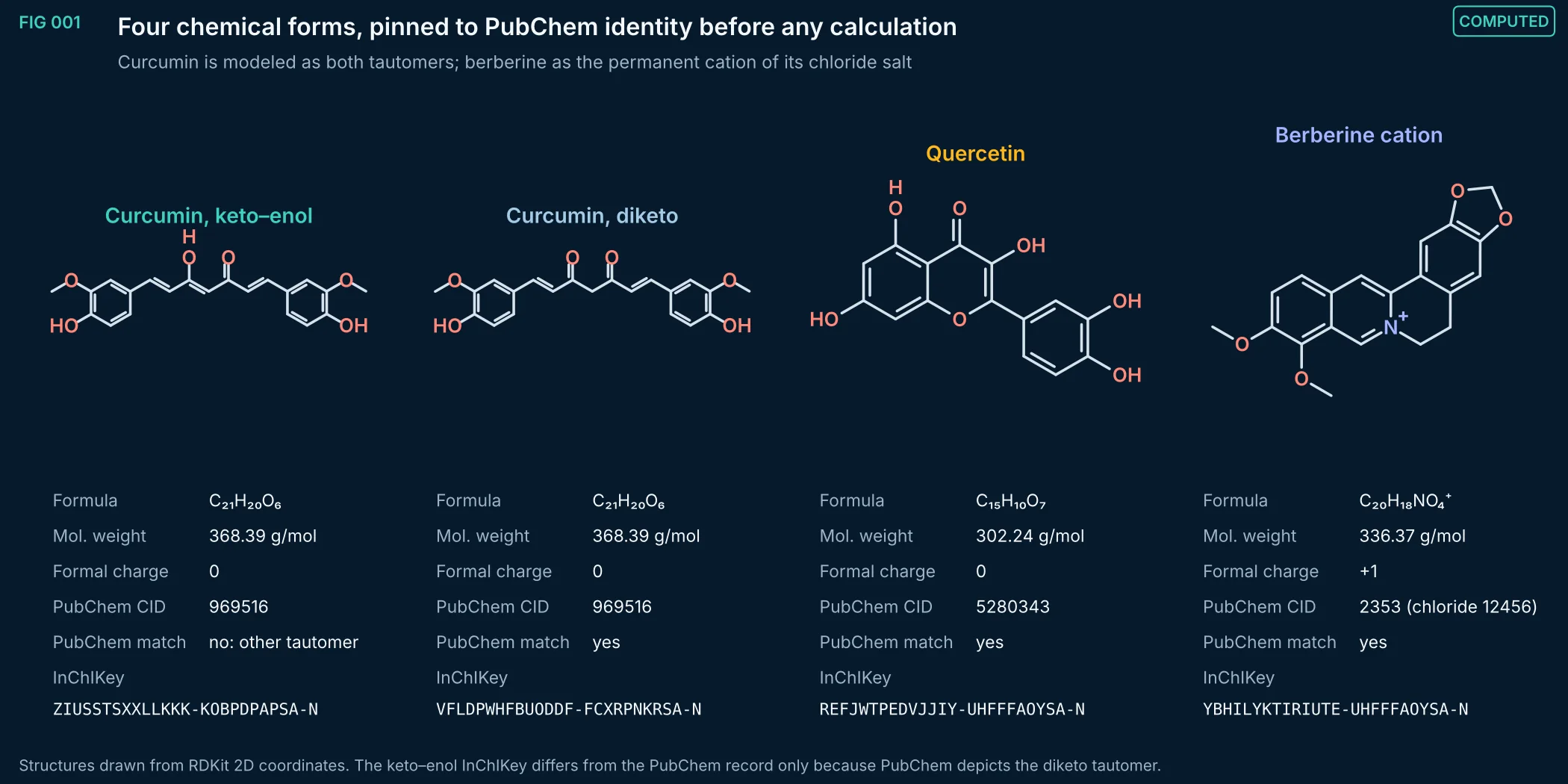
FIG 001Computed
Two-dimensional structures, formulas, molecular weights and InChIKeys of the four modeled forms. The curcumin diketo form, quercetin and the berberine cation reproduce the PubChem InChIKeys exactly; the Z keto–enol tautomer of curcumin is a deliberate second form, because crystal and solution studies place curcumin mainly in the enol form.
Method, sources and limits
- Method
- RDKit SMILES parsing, InChIKey generation and CoordGen 2D coordinates; values compared with PubChem PUG REST records retrieved November 5, 2026.
- Sources and code
- RDKit 2026.09.1 ETKDGv3 embedding (seed 20261105, no pruning) and MMFF94s minimization (maxIters 5000); scripts 01_molecular_structures/s01_compute.py and s01_export_minima.py. Structures from PubChem (CIDs 969516, 5280343, 2353).
- Supports
- Each calculation refers to a defined chemical form traceable to PubChem.
- Does not support
- Any statement about the composition of a commercial ingredient or extract.
- Limitations
- Identity checks confirm connectivity and tautomer, not purity or polymorph of any physical sample.
- Berberine is modeled without its chloride counter-ion except in the MD solvation boxes.
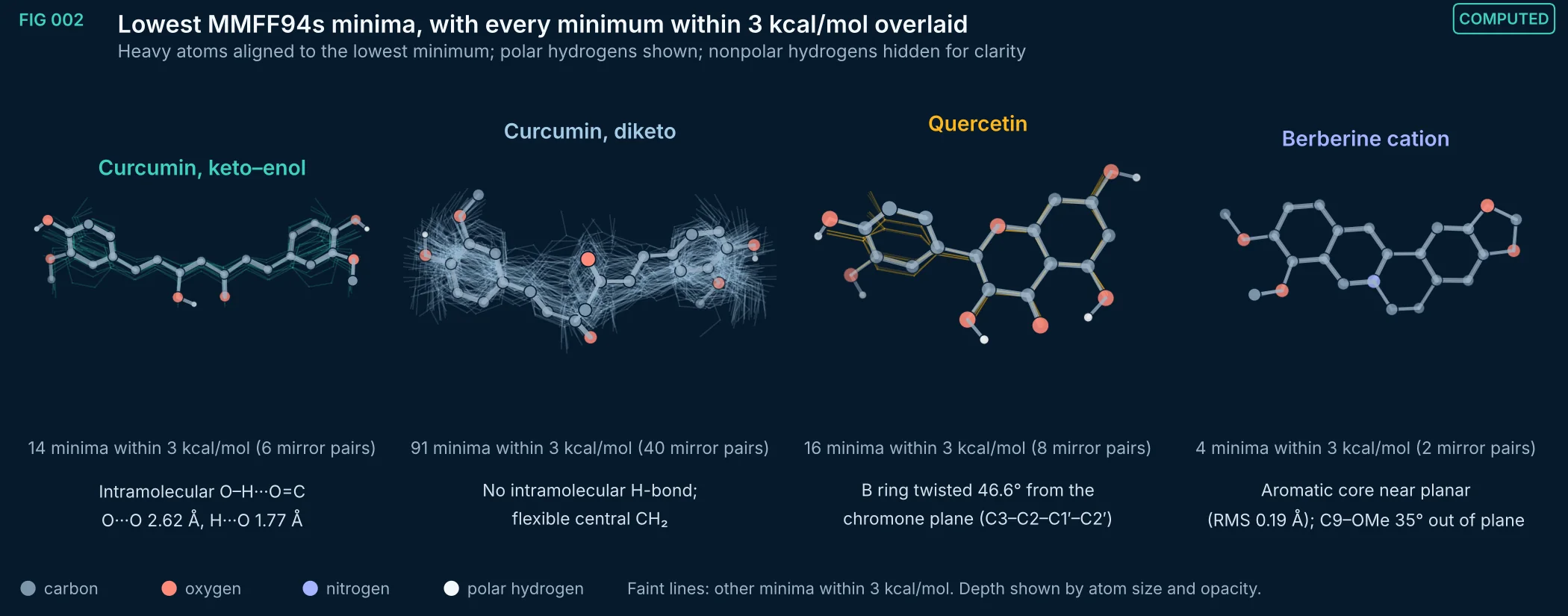
FIG 002Computed
Lowest-energy MMFF94s minimum of each form, projected on its principal axes, with all other unique minima within 3 kcal/mol overlaid as faint heavy-atom frames. The curcumin keto–enol minimum keeps the intramolecular O–H···O=C hydrogen bond; the diketo form has none. Quercetin's B ring is twisted relative to the chromone plane. Berberine's aromatic core is close to planar.
Method, sources and limits
- Method
- Unique minima (energy within 0.005 kcal/mol and heavy-atom RMSD below 0.15 Å treated as one) from 1,500 (curcumin), 400 (quercetin) or 200 (berberine) ETKDGv3 starts, MMFF94s-minimized; heavy-atom alignment to the lowest minimum; orthographic projection on principal axes.
- Sources and code
- RDKit 2026.09.1 ETKDGv3 embedding (seed 20261105, no pruning) and MMFF94s minimization (maxIters 5000); scripts 01_molecular_structures/s01_compute.py and s01_export_minima.py. Structures from PubChem (CIDs 969516, 5280343, 2353).
- Supports
- The geometric starting points used for solvation MD and descriptor calculations.
- Does not support
- Solution-phase conformer populations, tautomer ratios or crystal structures.
- Limitations
- Gas-phase force-field minima; solvent, counter-ion and crystal packing are absent.
- MMFF94s energies are not comparable between the two curcumin tautomers (different atom typing).
- A 3 kcal/mol window is a modeling convention, not a population at 300 K.
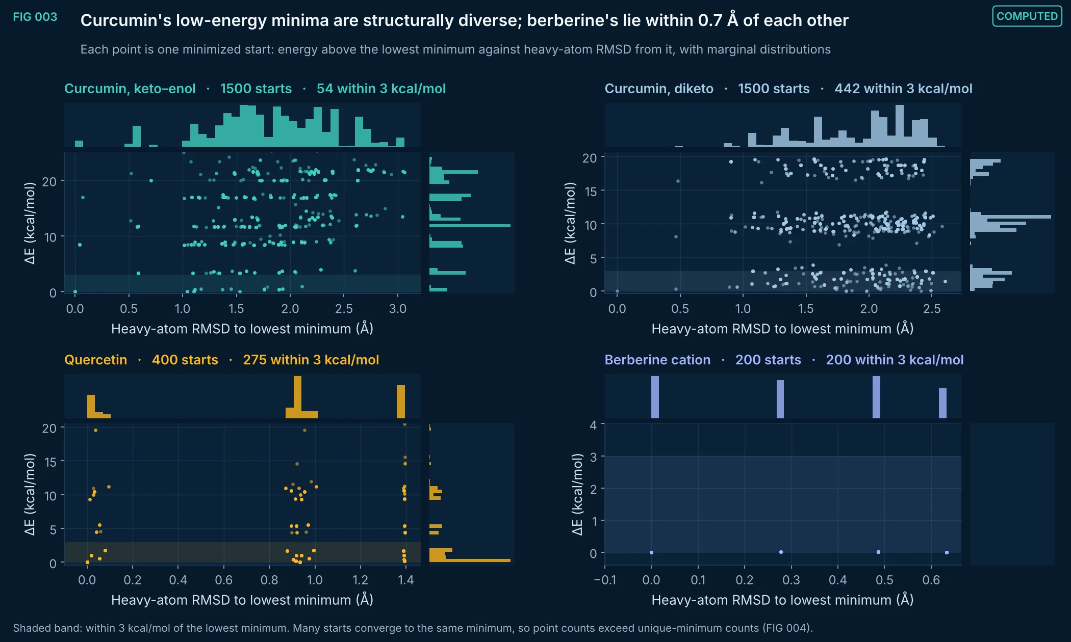
FIG 003Computed
Energy above the lowest MMFF94s minimum against heavy-atom RMSD to that minimum for every minimized start, with marginal histograms. Curcumin minima within 3 kcal/mol span RMSD values above 2 Å, so a single structure misrepresents it; berberine's 200 starts collapse onto four minima of essentially equal energy, all within 0.7 Å RMSD, two of them mirror images of the other two.
Method, sources and limits
- Method
- Same ensembles as FIG 002; symmetry-aware best RMSD (RDKit GetBestRMS) over heavy atoms.
- Sources and code
- RDKit 2026.09.1 ETKDGv3 embedding (seed 20261105, no pruning) and MMFF94s minimization (maxIters 5000); scripts 01_molecular_structures/s01_compute.py and s01_export_minima.py. Structures from PubChem (CIDs 969516, 5280343, 2353).
- Supports
- The need to carry conformer ensembles, not single structures, for curcumin into later calculations.
- Does not support
- Boltzmann populations in solution.
- Limitations
- Gas-phase MMFF94s energies.
- RMSD does not detect mirror-image conformers as identical (see FIG 004 notes).
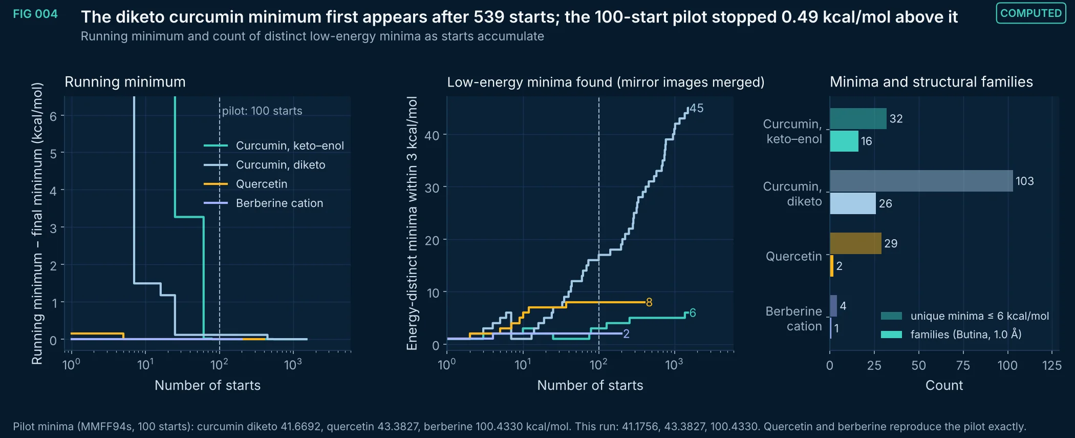
FIG 004Computed
Convergence of the conformer search. The curcumin diketo search reached its lowest minimum at start 539 of 1,500; the 100-start pilot's lowest diketo energy (41.6692 kcal/mol) is 0.49 kcal/mol above this run's (41.1756). Quercetin and berberine reach their minima within the first few starts and match the pilot to four decimals.
Method, sources and limits
- Method
- Running minimum over embedding order; energy-distinct minima (0.005 kcal/mol tolerance) within 3 kcal/mol of the running minimum; unique minima within 6 kcal/mol clustered with Butina at 1.0 Å heavy-atom RMSD.
- Sources and code
- RDKit 2026.09.1 ETKDGv3 embedding (seed 20261105, no pruning) and MMFF94s minimization (maxIters 5000); scripts 01_molecular_structures/s01_compute.py and s01_export_minima.py. Structures from PubChem (CIDs 969516, 5280343, 2353). Earlier 100-start run (version 0 of this calculation): conformer table kept in 00_provenance/.
- Supports
- That 100 starts were too few for curcumin and that 1,500 starts reached a stable minimum.
- Does not support
- Global-minimum certainty; QM or solution energetics.
- Limitations
- Embedding is stochastic and version-dependent; the 100-start run used a different RDKit build, so its individual starts are not reproducible.
- Unique-minimum counts include mirror-image (conformationally enantiomeric) pairs: Curcumin, keto–enol 14, Curcumin, diketo 46, Quercetin 14, Berberine cation 2 energy-degenerate pairs, each superimposable after inversion (RMSD below 0.001 Å).
- No search guarantees the global minimum.
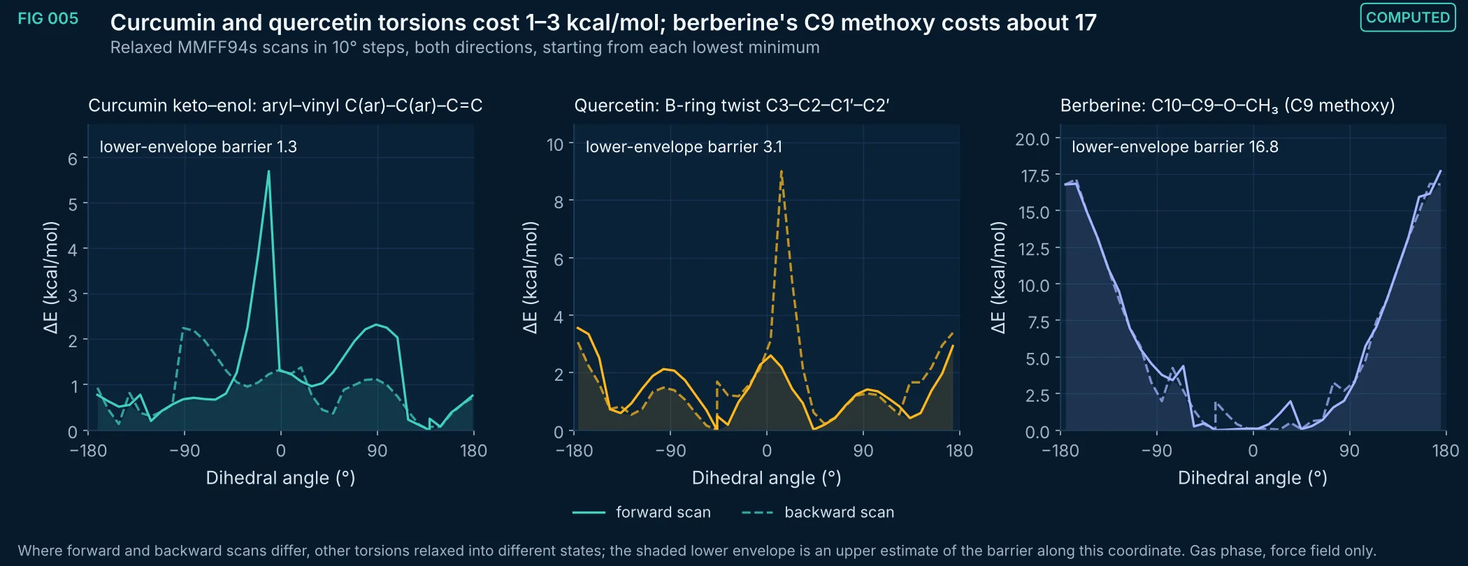
FIG 005Computed
Relaxed torsion scans (MMFF94s, 10° steps, restrained dihedral, all other coordinates minimized) in both directions from the lowest minimum. The curcumin aryl–vinyl and quercetin B-ring rotations are soft; berberine's C9 methoxy turns freely on the C10 side but is strongly hindered when the methyl is turned toward the ring-fusion side (C10–C9–O–CH₃ near 180°), next to the C8–H.
Method, sources and limits
- Method
- Dihedral set and restrained (force constant 1.0e4 kcal/mol/rad²) in RDKit MMFF94s, minimized to convergence, energy re-evaluated without the restraint; forward and backward sweeps of 360°.
- Sources and code
- RDKit 2026.09.1 ETKDGv3 embedding (seed 20261105, no pruning) and MMFF94s minimization (maxIters 5000); scripts 01_molecular_structures/s01_compute.py and s01_export_minima.py. Structures from PubChem (CIDs 969516, 5280343, 2353).
- Supports
- Qualitative ranking of torsional flexibility used to interpret conformer diversity (FIG 003).
- Does not support
- Quantitative rotational barriers or rates in solution.
- Limitations
- MMFF94s torsion parameters, not QM; barriers can differ by several kcal/mol from DFT.
- Gas phase; hysteresis between directions shows the scan is not a unique minimum-energy path.
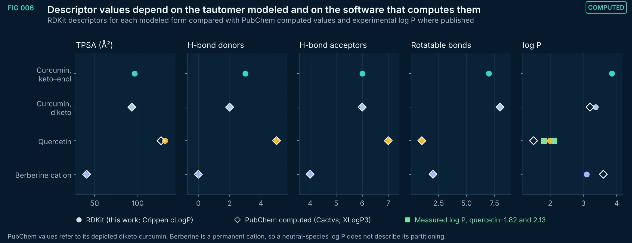
FIG 006Computed
RDKit descriptors of the four modeled forms beside PubChem computed values and published experimental log P for quercetin (1.82, Rothwell et al. 2005; 2.13, Sangster via PubChem). Moving curcumin from the diketo to the keto–enol form adds a hydrogen-bond donor and raises Crippen cLogP by about 0.5; RDKit and PubChem differ by about 4 Ų in quercetin TPSA.
Method, sources and limits
- Method
- RDKit 2026.09.1 descriptors (TPSA without S/P, Lipinski donors/acceptors, rotatable bonds, Crippen logP); PubChem PUG REST computed properties retrieved November 5, 2026.
- Sources and code
- RDKit 2026.09.1 ETKDGv3 embedding (seed 20261105, no pruning) and MMFF94s minimization (maxIters 5000); scripts 01_molecular_structures/s01_compute.py and s01_export_minima.py. Structures from PubChem (CIDs 969516, 5280343, 2353). Experimental quercetin log P: PubChem (Sangster) and Rothwell JA et al. J Agric Food Chem 2005.
- Supports
- The choice of tautomer and software must be fixed and reported for any descriptor-based model.
- Does not support
- Absorption, permeability or bioavailability predictions.
- Limitations
- Descriptors are 2D and conformer-independent.
- Computed log P values are estimates; only quercetin has a measured value here.
- Ionization (FIG 007) changes apparent distribution at physiological pH.
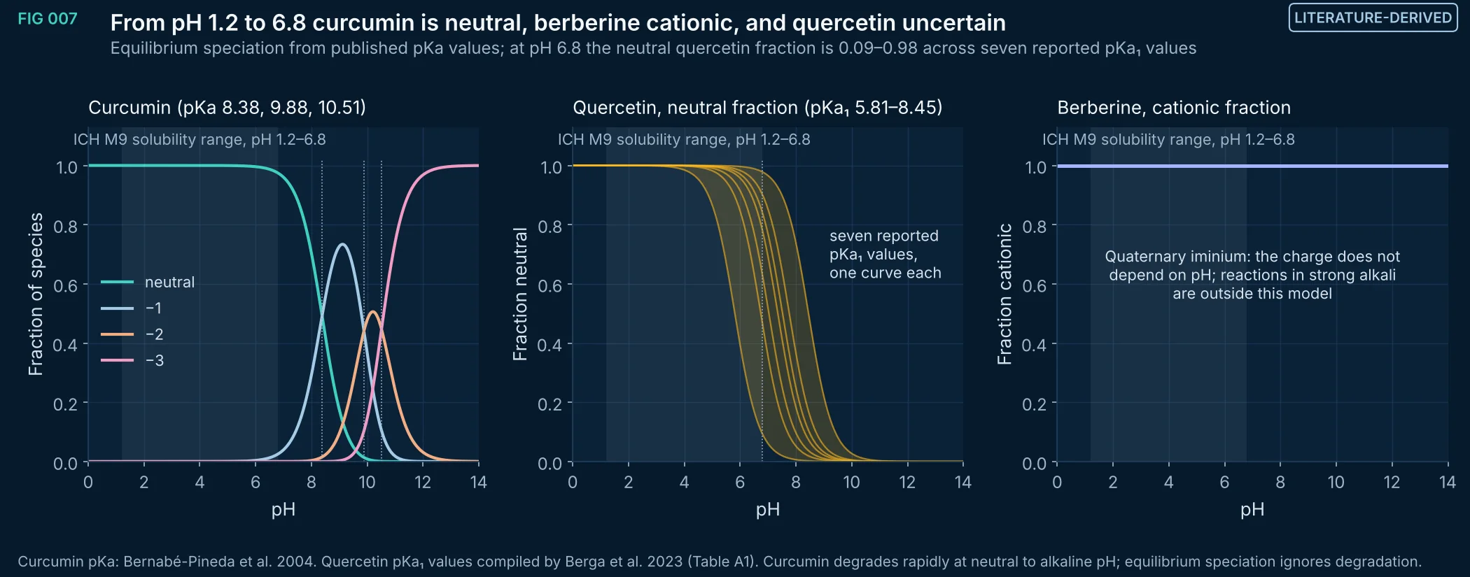
FIG 007Literature-derived
Equilibrium speciation versus pH. Curcumin (macroscopic pKa 8.38, 9.88, 10.51) is 97% neutral at pH 6.8. Seven published values of quercetin's first pKa (5.81 to 8.45) put its neutral fraction at pH 6.8 anywhere from 0.09 to 0.98. Berberine is a quaternary cation at every pH shown.
Method, sources and limits
- Method
- Henderson–Hasselbalch macroscopic speciation, sequential pKa values; quercetin first deprotonation only.
- Sources and code
- Curcumin: Bernabé-Pineda M et al. Spectrochim Acta A 2004;60:1091–1097, doi:10.1016/S1386-1425(03)00342-1. Quercetin: Berga M et al. Pharmaceuticals 2023;16(10):1407, Table A1, doi:10.3390/ph16101407. pH range: ICH M9 (2019) biopharmaceutics classification, solubility over pH 1.2–6.8. Script 01_molecular_structures/s01_figures.py.
- Supports
- Which species should be modeled in each pH region; the need to resolve quercetin's pKa experimentally before pH-dependent modeling.
- Does not support
- Solubility at a given pH; absorption predictions.
- Limitations
- Macroscopic pKa values; microspecies and tautomer-specific ionization are not resolved.
- Temperature and ionic strength of the source measurements differ.
- Degradation of curcumin at pH ≥ 7 is not modeled.
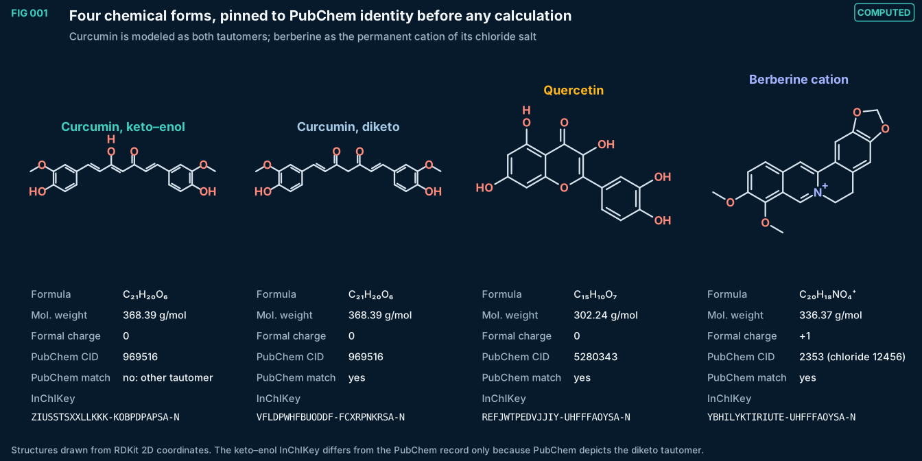
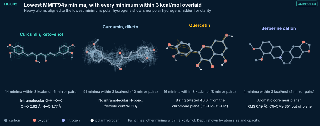
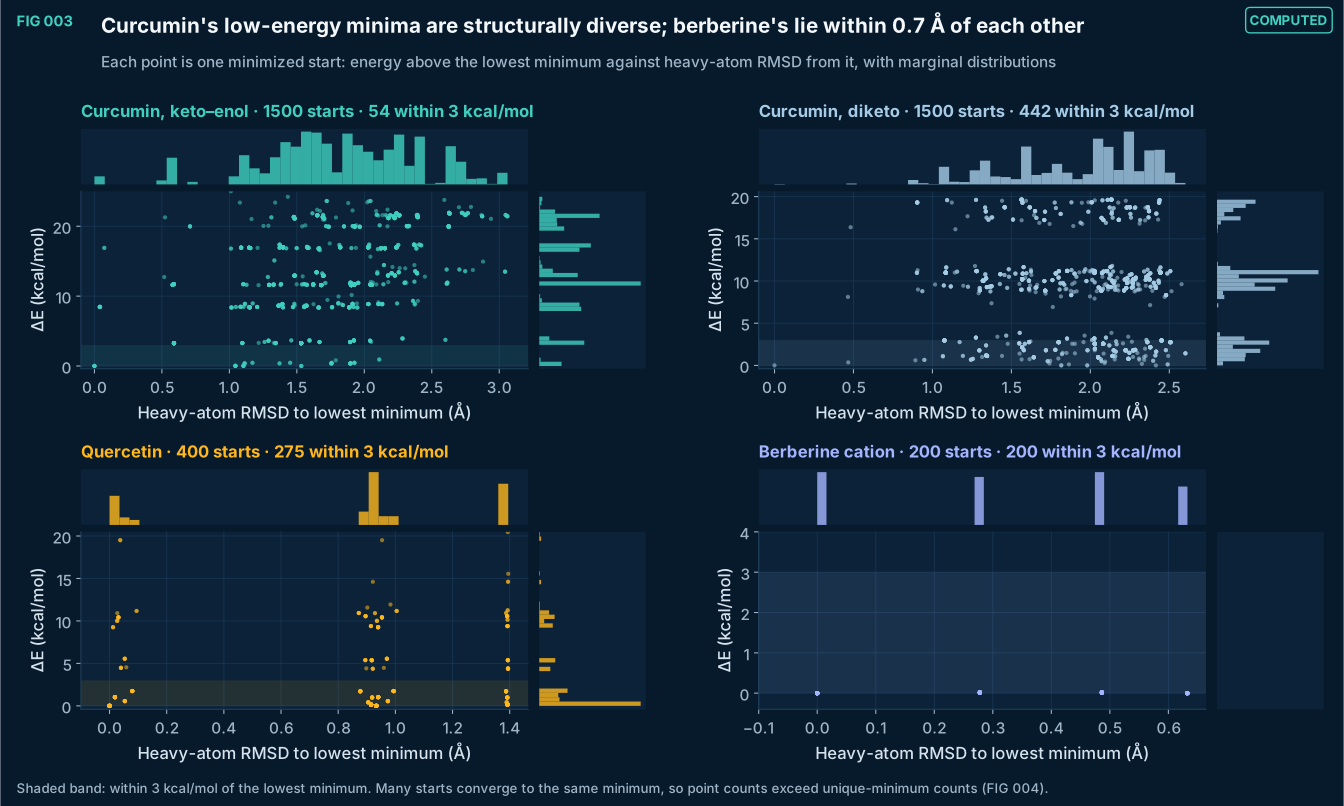
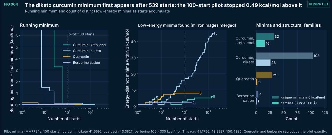
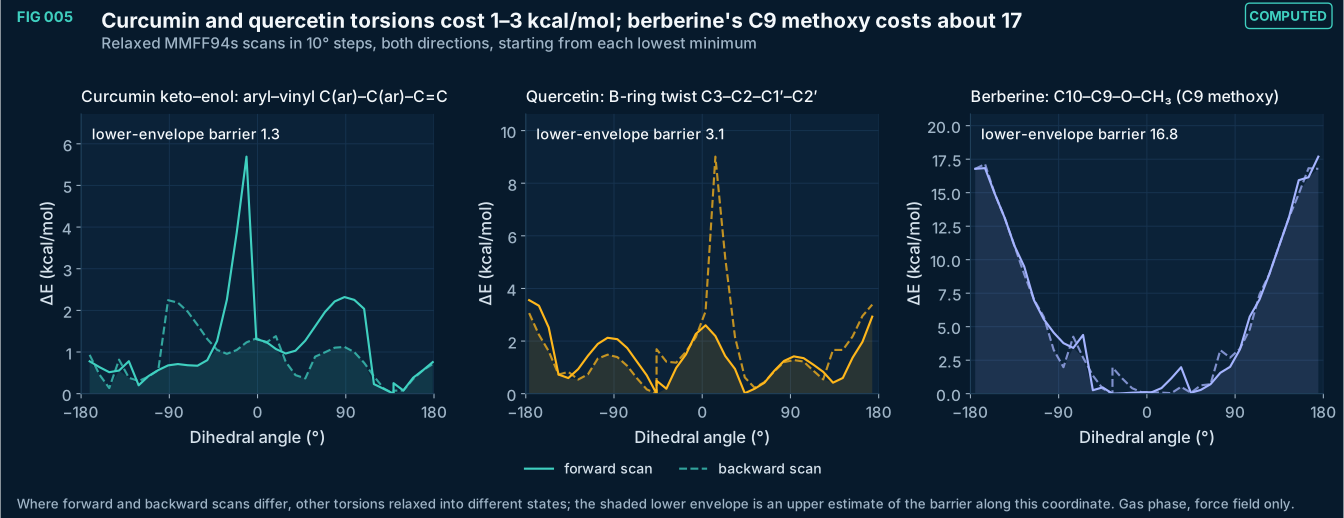
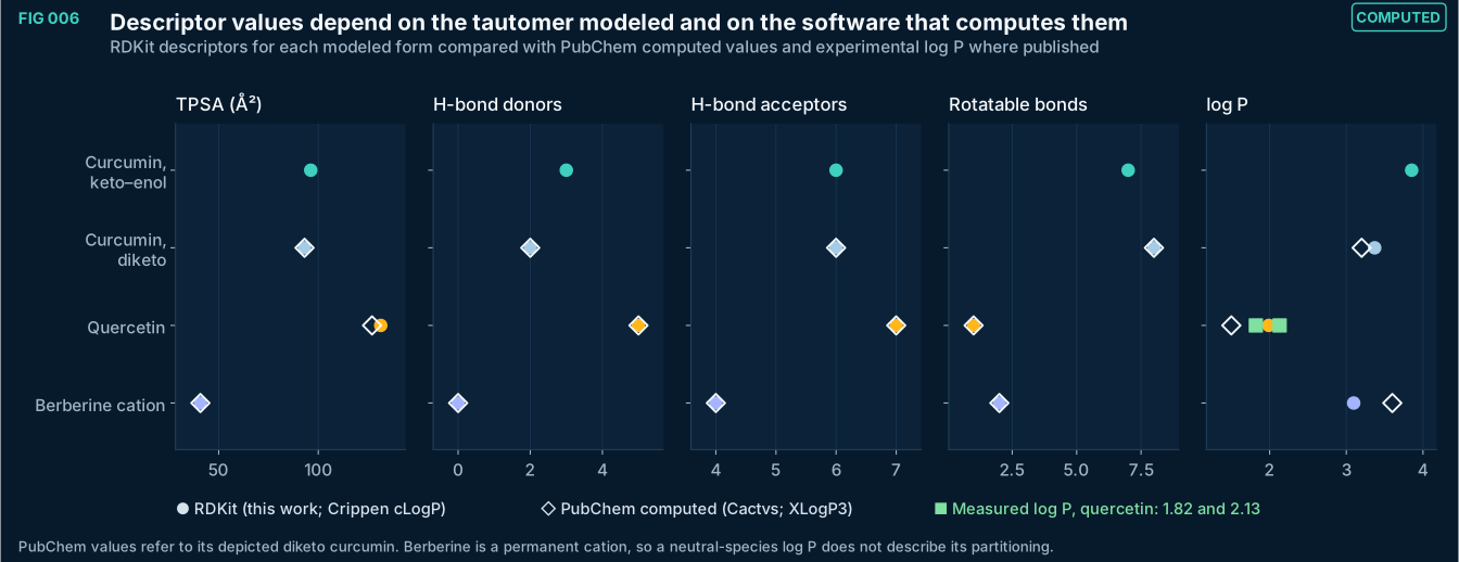
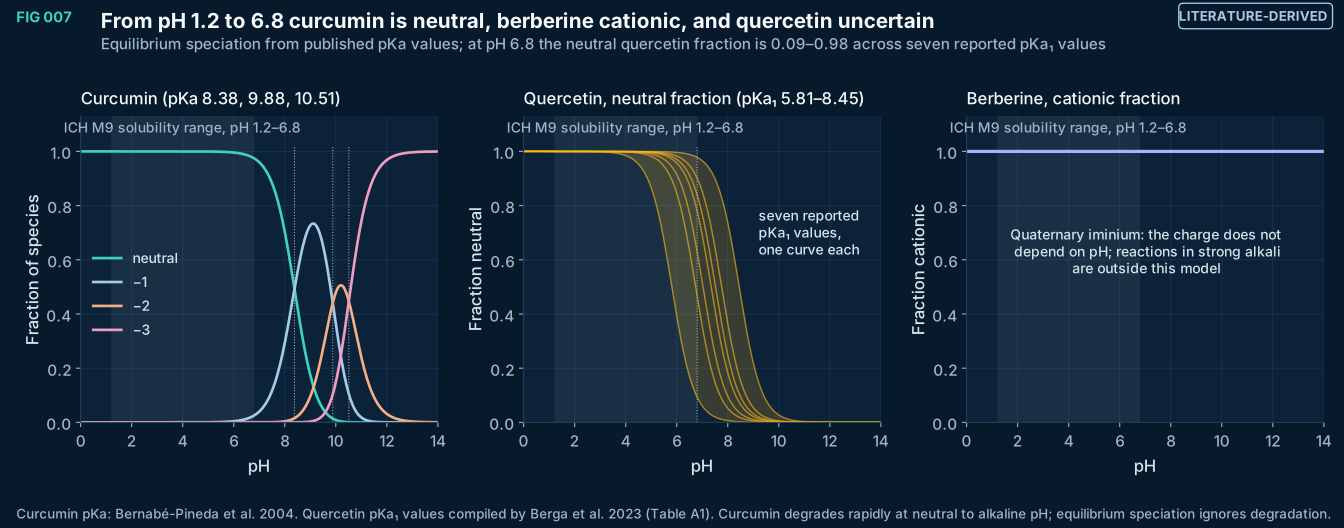
FIG 008–010
Molecular dynamics
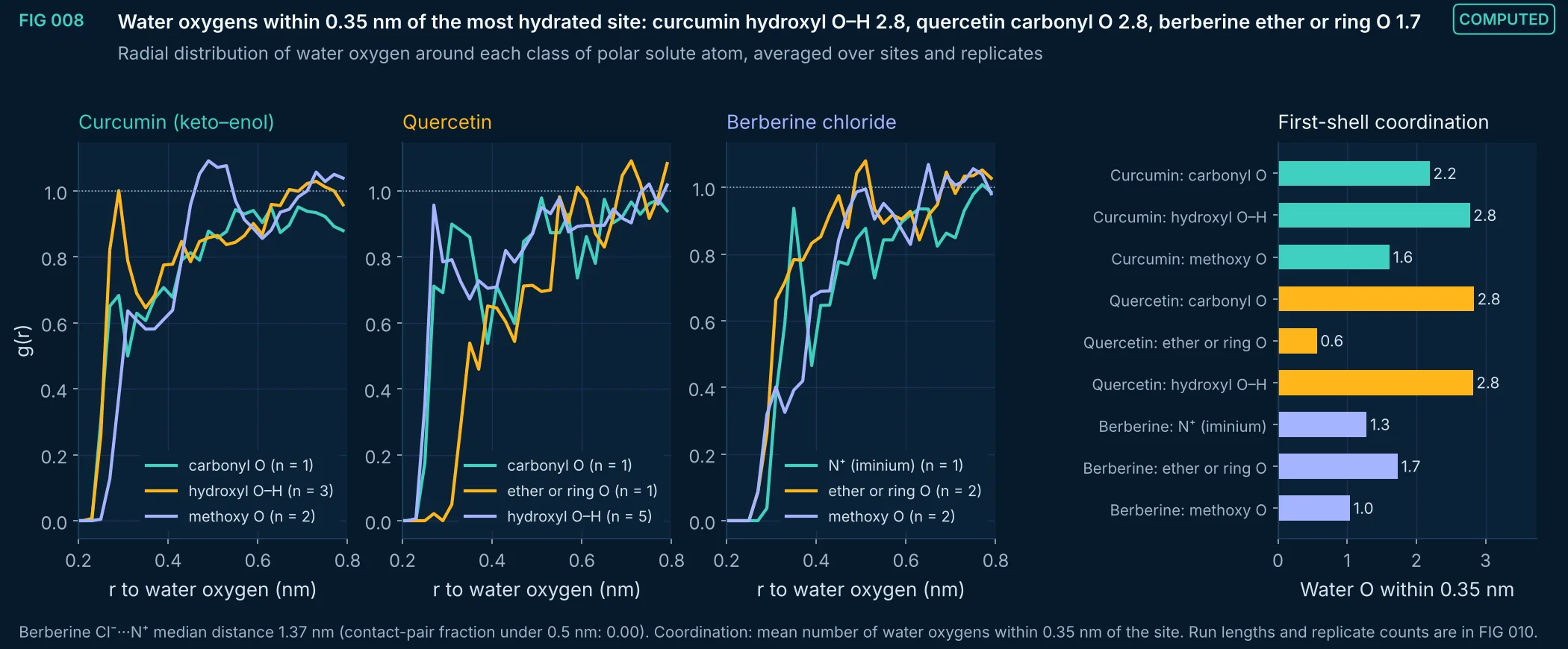
FIG 008Computed
Solvation structure from explicit-solvent molecular dynamics with MMFF94s: radial distribution functions of water oxygen around the polar atoms of each solute, and first-shell coordination numbers. Coordination differs several-fold between site types; in curcumin the hydroxyl that takes part in the intramolecular enol hydrogen bond is partly shielded from water (FIG 009). These are the solute–solvent contacts that continuum solubility models average away.
Method, sources and limits
- Method
- g(r) from minimum-image distances in the cubic NPT box, frame-wise box length, 0.02 nm bins; averaged over equivalent sites and over replicates; coordination counted within 0.35 nm.
- Sources and code
- MMFF94s in OpenMM 8.6.1 (custom forces verified against RDKit), PME, Langevin 300 K, Monte Carlo barostat 1 bar, 2 fs; frames every 0.5 ps. Scripts 02_force_fields_and_MD/md_run.py and md_figs.py.
- Supports
- Which solute sites dominate hydration, as input to solubility and permeability reasoning.
- Does not support
- Quantitative hydration free energies or solubilities.
- Limitations
- Short trajectories (tens of picoseconds per replicate): adequate for first-shell structure and fast hydrogen-bond dynamics, not for conformational sampling or slow events.
- MMFF94s with its own water parameters, not a dedicated water model such as TIP3P or OPC; water density and structure differ from experiment.
- One solute molecule per box; no concentration, aggregation or counter-ion pairing statistics beyond what a single ion shows.
Vector (SVG) · Full-size image · data (coordination) (CSV) · data (rdf) (CSV)
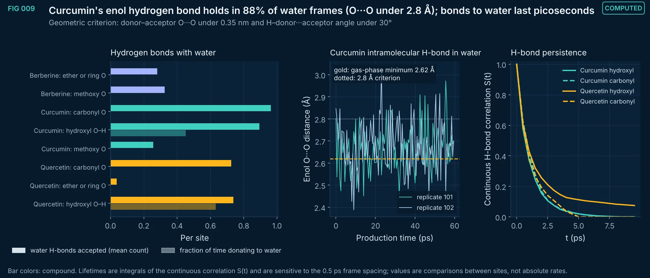
FIG 009Computed
Hydrogen bonding between each solute and water. Hydroxyl groups both donate and accept; carbonyl and ether oxygens only accept. In curcumin the intramolecular O–H···O=C bond of the keto–enol form persists in water for most of the trajectory, which keeps that hydroxyl partly unavailable to the solvent. Solute–water hydrogen bonds persist for only a few picoseconds.
Method, sources and limits
- Method
- Geometric hydrogen-bond criterion on every frame; per-site occupancy; continuous correlation S(t) with 0.5 ps resolution; enol O···O distance time series.
- Sources and code
- MMFF94s in OpenMM 8.6.1 (custom forces verified against RDKit), PME, Langevin 300 K, Monte Carlo barostat 1 bar, 2 fs; frames every 0.5 ps. Scripts 02_force_fields_and_MD/md_run.py and md_figs.py.
- Supports
- Which groups of each molecule interact with water and how long those contacts last.
- Does not support
- Solubility values or tautomer populations in water.
- Limitations
- Short trajectories (tens of picoseconds per replicate): adequate for first-shell structure and fast hydrogen-bond dynamics, not for conformational sampling or slow events.
- MMFF94s with its own water parameters, not a dedicated water model such as TIP3P or OPC; water density and structure differ from experiment.
- One solute molecule per box; no concentration, aggregation or counter-ion pairing statistics beyond what a single ion shows.
- Geometric criteria are conventions; changing the cutoffs changes absolute counts.
Vector (SVG) · Full-size image · data (lifetimes) (CSV) · data (occupancy) (CSV)
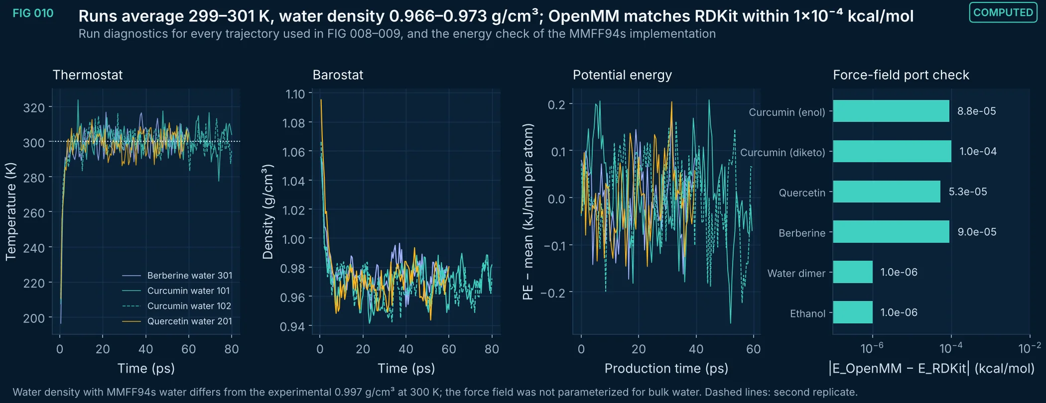
FIG 010Computed
Quality checks for the explicit-solvent trajectories: thermostat and barostat behavior, potential-energy stationarity during production, and the agreement between the OpenMM implementation of MMFF94s and RDKit's reference implementation for every molecule, including a water dimer that tests intermolecular terms.
Method, sources and limits
- Method
- State data every 0.5 ps; production means and SDs; linear drift and 4-block means of potential energy; single-point energy comparison on identical coordinates.
- Sources and code
- MMFF94s in OpenMM 8.6.1 (custom forces verified against RDKit), PME, Langevin 300 K, Monte Carlo barostat 1 bar, 2 fs; frames every 0.5 ps. Scripts 02_force_fields_and_MD/md_run.py and md_figs.py. Verification: 02_force_fields_and_MD/verify_mmff.py.
- Supports
- That the trajectories are equilibrated in temperature and density over their length and that the force field is implemented correctly.
- Does not support
- Convergence of slow conformational transitions.
- Limitations
- Short trajectories (tens of picoseconds per replicate): adequate for first-shell structure and fast hydrogen-bond dynamics, not for conformational sampling or slow events.
- MMFF94s with its own water parameters, not a dedicated water model such as TIP3P or OPC; water density and structure differ from experiment.
- One solute molecule per box; no concentration, aggregation or counter-ion pairing statistics beyond what a single ion shows.
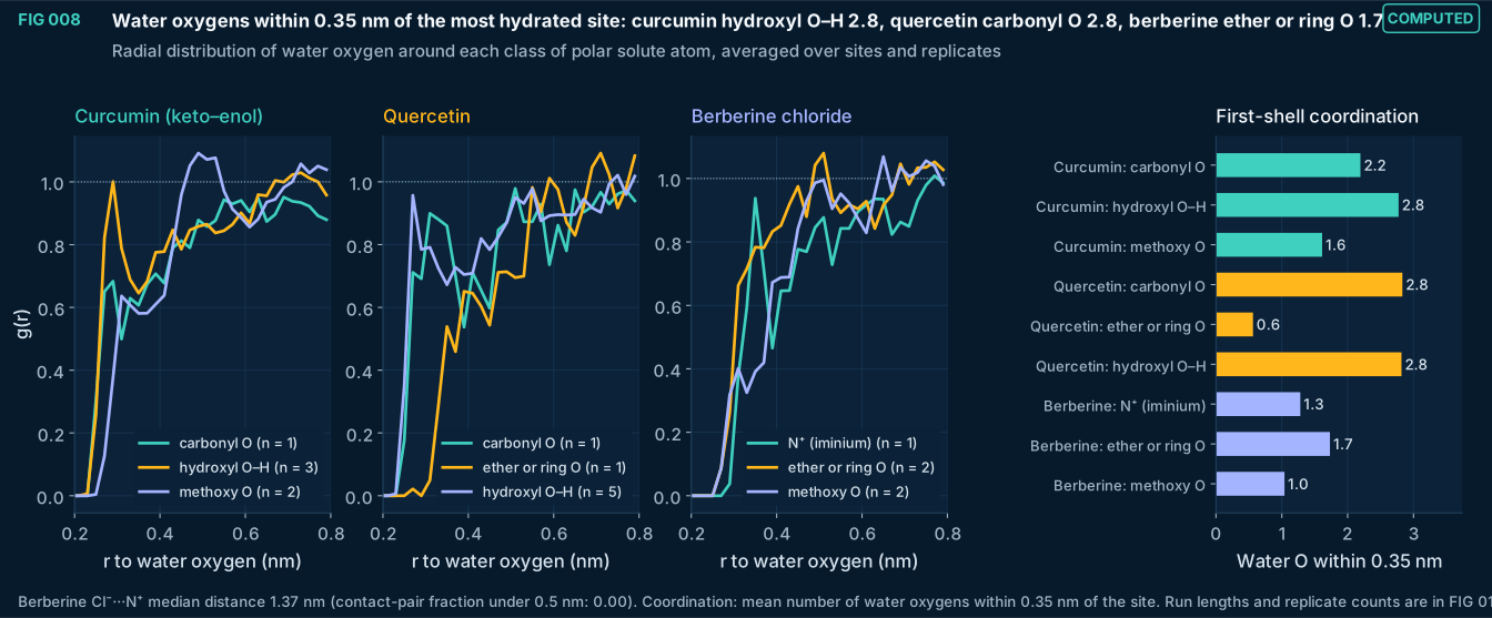
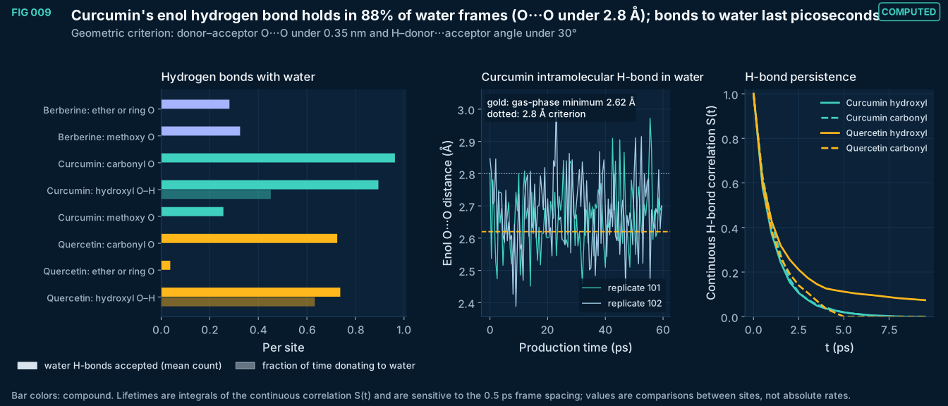
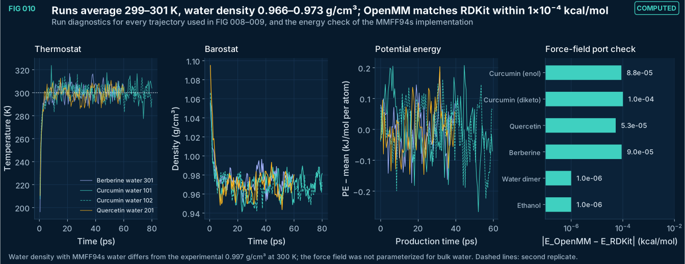
FIG 011–015
Solubility and solvent selection
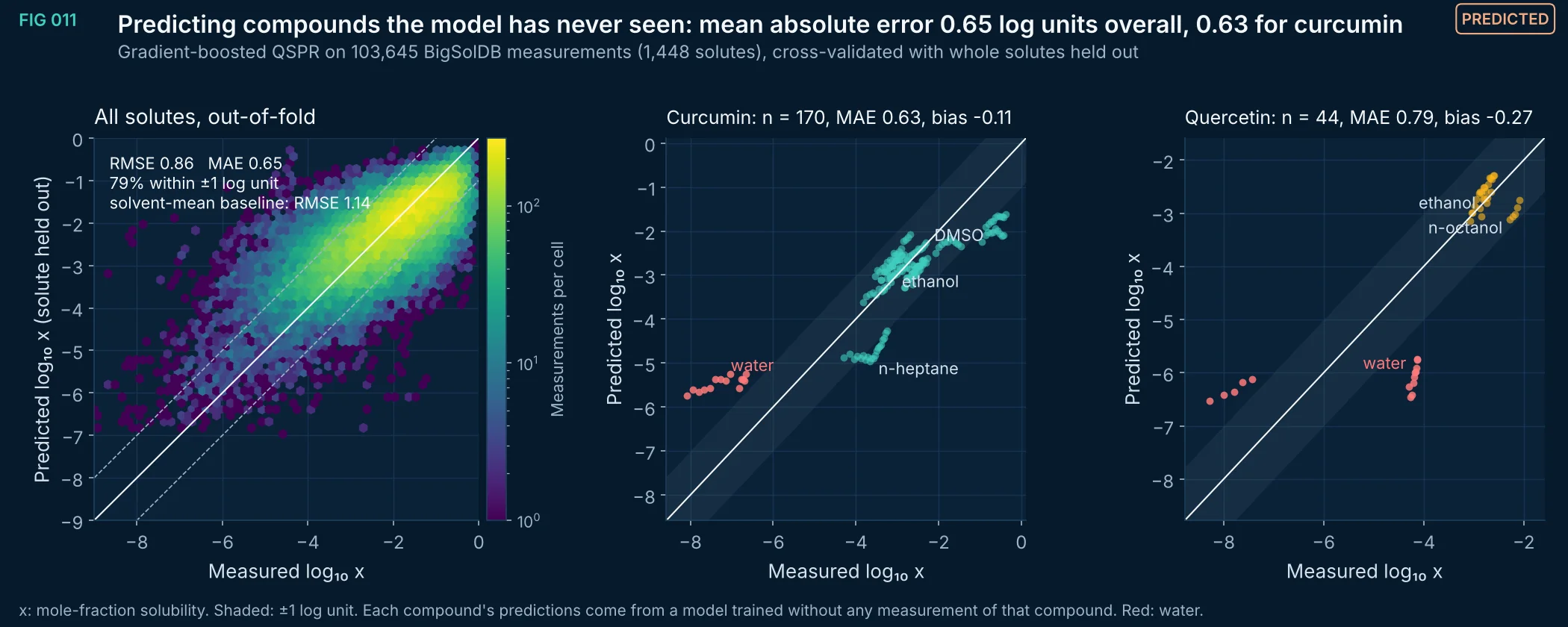
FIG 011Predicted
Out-of-fold predictions of a gradient-boosted QSPR model trained on BigSolDB 2.0, with every measurement of a solute held out together (GroupKFold, 5 folds). Across 1,448 solutes the RMSE is 0.86 log₁₀ units against 1.14 for a solvent-mean baseline. Curcumin (MAE 0.63) and quercetin (MAE 0.79) were predicted by models that never saw them.
Method, sources and limits
- Method
- HistGradientBoostingRegressor(max_iter=250, lr=0.1, max_leaf_nodes=63, min_samples_leaf=30, l2=1.0); features: 13 RDKit descriptors of solute and solvent, 256-bit Morgan count fingerprint (radius 2) of the solute, 1000/T. Target log₁₀ mole fraction. GroupKFold(5) by solute SMILES.
- Sources and code
- Krasnov L. et al. BigSolDB 2.0, Zenodo (CSV v2.0; SHA256 879f55f3…). Curcumin rows: Cui et al. J Mol Liq 2021 (10.1016/j.molliq.2021.116795); Shen et al. J Chem Thermodyn 2019 (10.1016/j.jct.2018.11.022); Fluid Phase Equilib 2021 (10.1016/j.fluid.2020.112917). Quercetin rows: Razmara et al. J Chem Eng Data 2010 (10.1021/je9010757); Zhang et al. J Mol Liq 2017 (10.1016/j.molliq.2016.11.036); Montenegro et al. J Chem Thermodyn 2025;203:107434 (10.1016/j.jct.2024.107434). Scripts 03_thermodynamics_CAMD/thermo_compute.py and thermo_figs.py.
- Supports
- Solvent screening and ranking before measurement; typical expected error of about one log unit.
- Does not support
- Replacing measured solubility for formulation or process design.
- Solubility of mixtures, extracts or salts.
- Limitations
- Data-driven correlation; no thermodynamic constraint, so predictions outside the chemical space of BigSolDB are unreliable.
- Polymorph, purity and method differences in the source data are not represented.
- Error is reported per measurement; compounds with many rows weigh more in the overall RMSE.
Vector (SVG) · Full-size image · data (case_rows) (CSV) · data (oof_sample) (CSV)
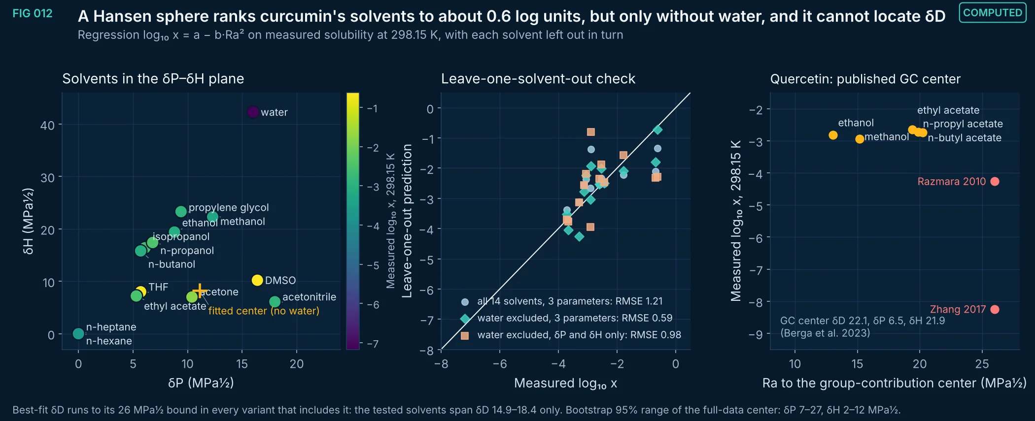
FIG 012Computed
Curcumin solubility at 298.15 K (van 't Hoff interpolation of the measured series) regressed on the Hansen distance Ra to a fitted center. Without water, leave-one-solvent-out RMSE is 0.59 log₁₀ units; including water it rises to 1.21. The dispersion coordinate δD is not identifiable from these solvents. For quercetin, the published group-contribution center orders the organic solvents only weakly and cannot be tested in water, where the two datasets disagree.
Method, sources and limits
- Method
- Least-squares fit of log₁₀ x = a − b·Ra², Ra² = 4(δD−δD₀)² + (δP−δP₀)² + (δH−δH₀)², multi-start; leave-one-out refits; 300-sample bootstrap over solvents. m-Xylene omitted (no Hansen values collected).
- Sources and code
- Krasnov L. et al. BigSolDB 2.0, Zenodo (CSV v2.0; SHA256 879f55f3…). Curcumin rows: Cui et al. J Mol Liq 2021 (10.1016/j.molliq.2021.116795); Shen et al. J Chem Thermodyn 2019 (10.1016/j.jct.2018.11.022); Fluid Phase Equilib 2021 (10.1016/j.fluid.2020.112917). Quercetin rows: Razmara et al. J Chem Eng Data 2010 (10.1021/je9010757); Zhang et al. J Mol Liq 2017 (10.1016/j.molliq.2016.11.036); Montenegro et al. J Chem Thermodyn 2025;203:107434 (10.1016/j.jct.2024.107434). Hansen CM. Hansen Solubility Parameters: A User's Handbook, 2nd ed. CRC Press, 2007; n-hexane: Carré et al. 2024. Berga M et al. Pharmaceuticals 2023;16(10):1407, Table A3 (group-contribution estimate), doi:10.3390/ph16101407 Scripts 03_thermodynamics_CAMD/thermo_compute.py and thermo_figs.py.
- Supports
- Coarse solvent ranking; the need for solvents with higher δD to constrain the center.
- Does not support
- A definitive Hansen parameter set for curcumin or quercetin.
- Prediction of water solubility.
- Limitations
- A Hansen sphere is a correlative model; it ignores temperature, solute melting and specific association.
- Only 13–14 solvents; the center is poorly constrained (wide bootstrap range).
- Values at 298.15 K are interpolated from each published series; where two sources exist their logarithms are averaged.
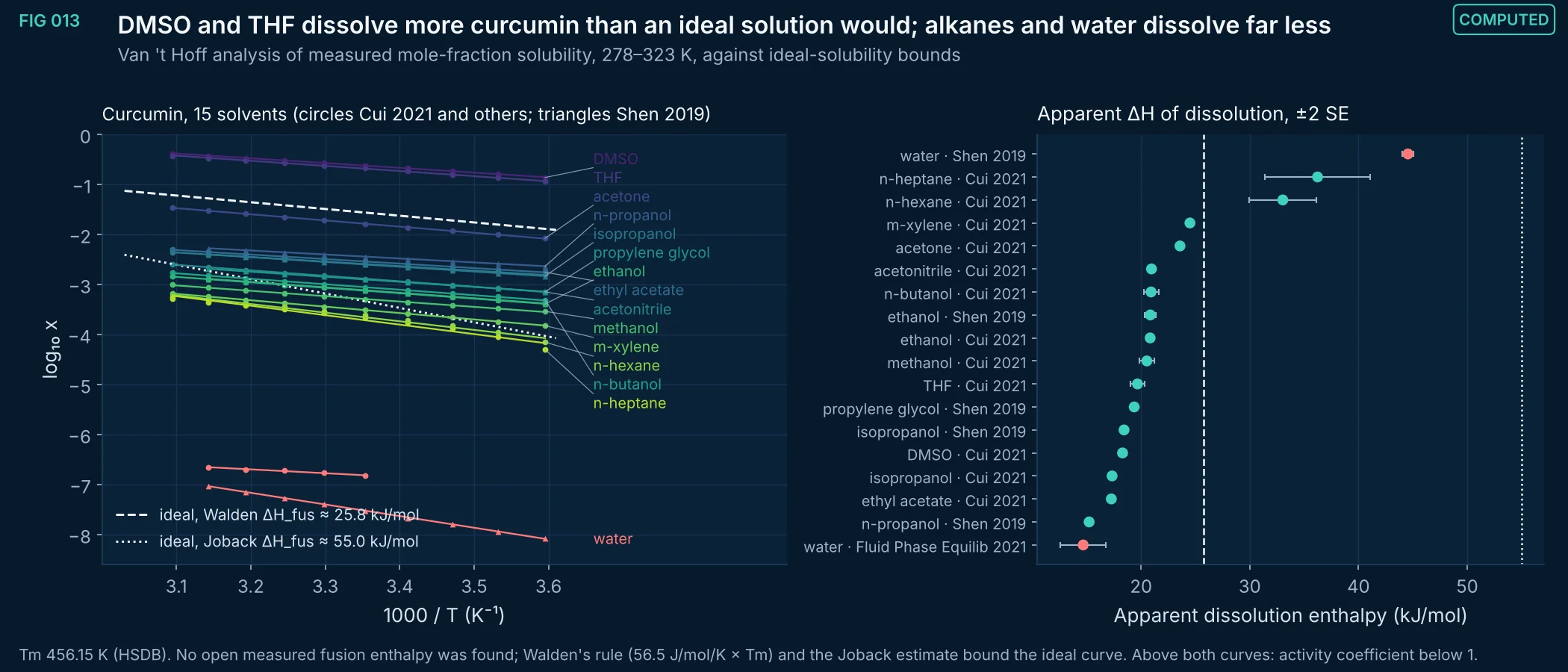
FIG 013Computed
Mole-fraction solubility of curcumin against inverse temperature for 15 solvents, with linear van 't Hoff fits and two ideal-solubility curves that bracket the unknown fusion enthalpy. DMSO and THF lie above both ideal curves, so curcumin's activity coefficient in them is below 1 (favorable specific interactions); n-heptane, n-hexane and water lie far below. The right panel gives each series' apparent dissolution enthalpy; the two water series disagree by about 30 kJ/mol.
Method, sources and limits
- Method
- Ordinary least squares of ln x on 1/T per solvent and source; ΔH_app = −R·slope; ideal solubility ln x = −ΔH_fus/R (1/T − 1/T_m), neglecting ΔC_p.
- Sources and code
- Krasnov L. et al. BigSolDB 2.0, Zenodo (CSV v2.0; SHA256 879f55f3…). Curcumin rows: Cui et al. J Mol Liq 2021 (10.1016/j.molliq.2021.116795); Shen et al. J Chem Thermodyn 2019 (10.1016/j.jct.2018.11.022); Fluid Phase Equilib 2021 (10.1016/j.fluid.2020.112917). Quercetin rows: Razmara et al. J Chem Eng Data 2010 (10.1021/je9010757); Zhang et al. J Mol Liq 2017 (10.1016/j.molliq.2016.11.036); Montenegro et al. J Chem Thermodyn 2025;203:107434 (10.1016/j.jct.2024.107434). Tm: 183 °C, HSDB via PubChem (CRC: 456.15 K). Joback estimate via the chemicals 1.5.2 library. Scripts 03_thermodynamics_CAMD/thermo_compute.py and thermo_figs.py.
- Supports
- The solvent classes that interact favorably with curcumin; the internal consistency of each published series.
- Does not support
- Absolute activity coefficients; extraction yields from plant material.
- Limitations
- Fusion enthalpy is estimated, not measured; the ideal curve could lie anywhere between the two bounds or outside them.
- Apparent enthalpies assume constant ΔH over 278–323 K and no change of the solid phase (solvates or polymorph changes are not checked).
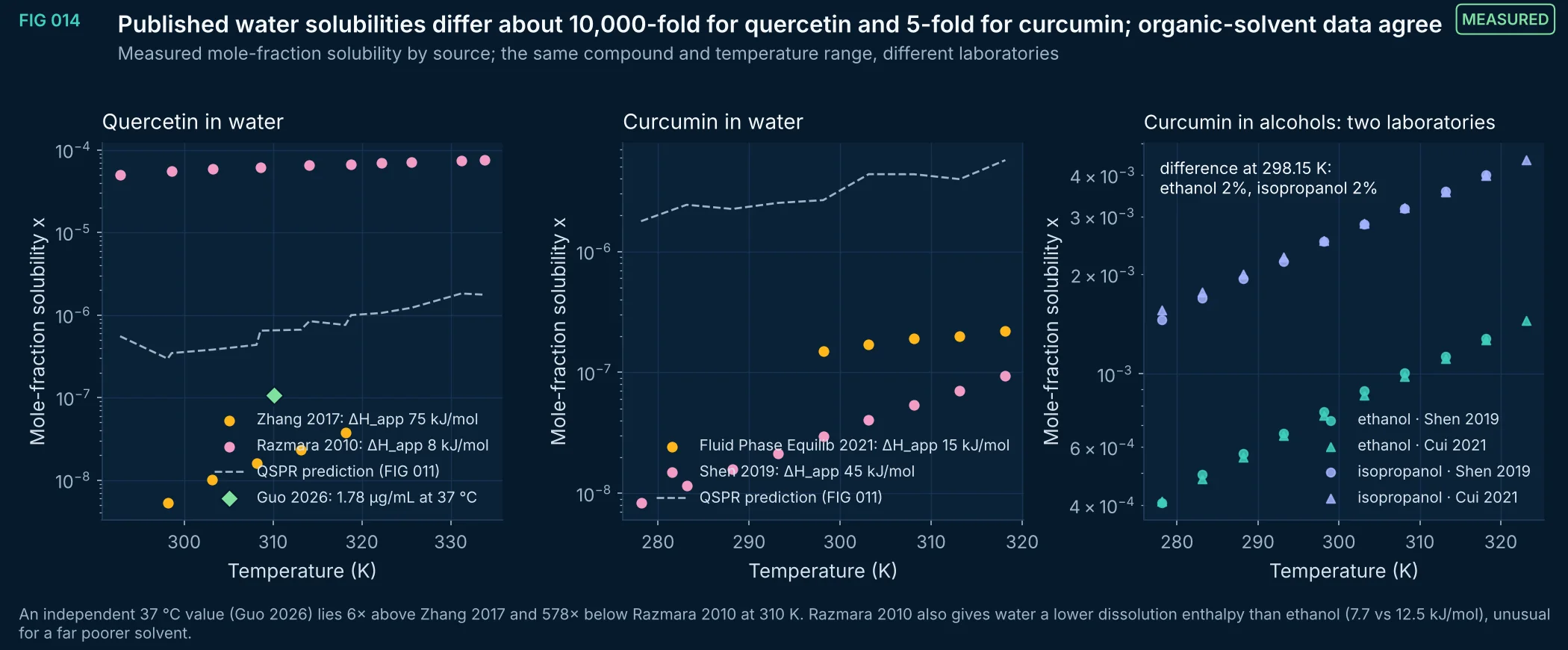
FIG 014Measured
Water solubility of quercetin from two laboratories differs about 10,000-fold at 298.15 K (van 't Hoff interpolation), and that of curcumin about 5-fold, while two laboratories' curcumin data in ethanol and isopropanol agree within a few percent. Water solubility is the quantity most often quoted for these compounds and the least reproducible here.
Method, sources and limits
- Method
- Published measurements as compiled in BigSolDB 2.0; ratios from per-source van 't Hoff fits at 298.15 K; QSPR line from FIG 011 for reference.
- Sources and code
- Krasnov L. et al. BigSolDB 2.0, Zenodo (CSV v2.0; SHA256 879f55f3…). Curcumin rows: Cui et al. J Mol Liq 2021 (10.1016/j.molliq.2021.116795); Shen et al. J Chem Thermodyn 2019 (10.1016/j.jct.2018.11.022); Fluid Phase Equilib 2021 (10.1016/j.fluid.2020.112917). Quercetin rows: Razmara et al. J Chem Eng Data 2010 (10.1021/je9010757); Zhang et al. J Mol Liq 2017 (10.1016/j.molliq.2016.11.036); Montenegro et al. J Chem Thermodyn 2025;203:107434 (10.1016/j.jct.2024.107434). Independent 37 °C quercetin value: Guo et al. Pharmaceuticals 2026;19(10):1625, doi:10.3390/ph19101625. Scripts 03_thermodynamics_CAMD/thermo_compute.py and thermo_figs.py.
- Supports
- Treating aqueous solubility of both compounds as uncertain by orders of magnitude until remeasured under controlled solid form and pH.
- Does not support
- Choosing either published water value for formulation design.
- Limitations
- Sources differ in method (shake-flask, analytical finish), solid form and equilibration time; these details were not re-examined from the full texts.
- The QSPR line is itself trained on public data that include one of the conflicting series' peers and cannot arbitrate.
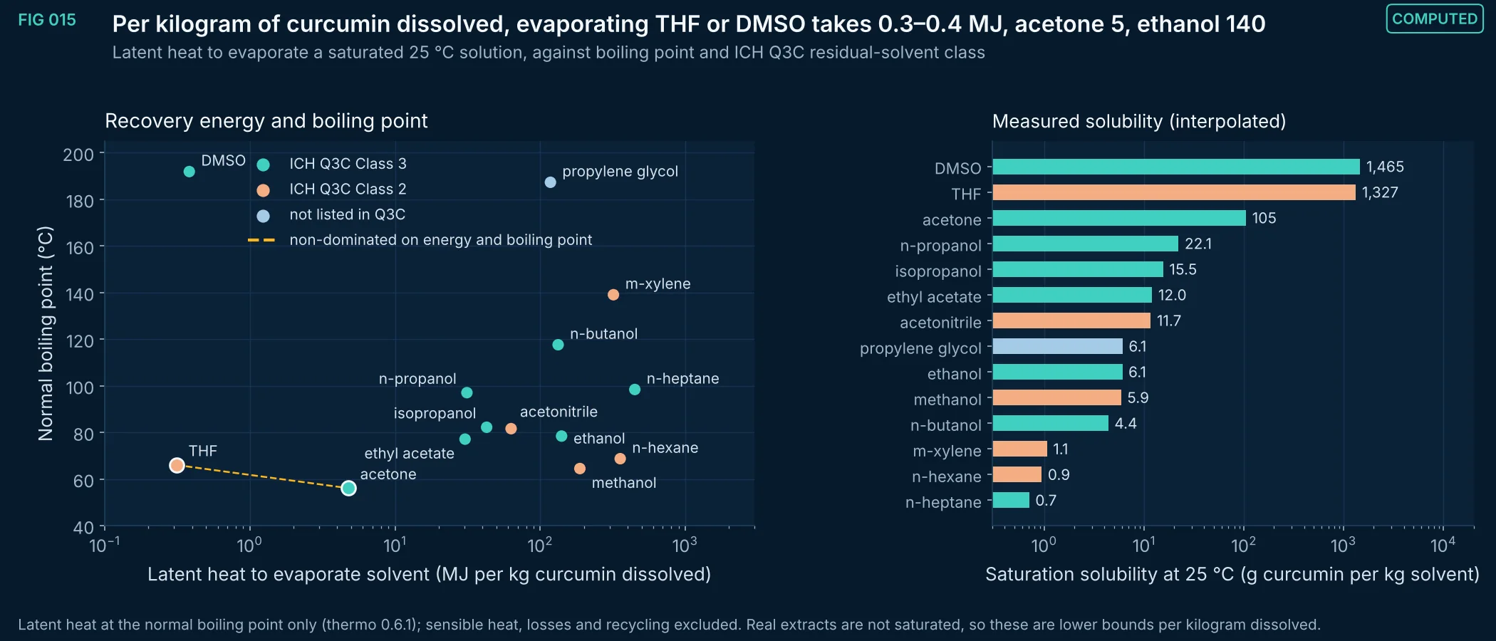
FIG 015Computed
For each solvent with measured curcumin solubility, the mass of solvent needed to dissolve 1 kg of curcumin at saturation (25 °C) times its enthalpy of vaporization, against boiling point, colored by ICH Q3C class. THF and DMSO need 0.3–0.4 MJ per kg dissolved because curcumin is very soluble in them, but THF is Class 2 and DMSO boils near 190 °C. Acetone is the lowest-energy Class 3 solvent with a low boiling point.
Method, sources and limits
- Method
- kg solvent per kg solute = (1 − x)/x · M_solvent/M_curcumin at the interpolated 298.15 K solubility; energy = that mass × ΔH_vap(T_b). Non-dominated set on (energy, boiling point).
- Sources and code
- Krasnov L. et al. BigSolDB 2.0, Zenodo (CSV v2.0; SHA256 879f55f3…). Curcumin rows: Cui et al. J Mol Liq 2021 (10.1016/j.molliq.2021.116795); Shen et al. J Chem Thermodyn 2019 (10.1016/j.jct.2018.11.022); Fluid Phase Equilib 2021 (10.1016/j.fluid.2020.112917). Quercetin rows: Razmara et al. J Chem Eng Data 2010 (10.1021/je9010757); Zhang et al. J Mol Liq 2017 (10.1016/j.molliq.2016.11.036); Montenegro et al. J Chem Thermodyn 2025;203:107434 (10.1016/j.jct.2024.107434). ICH Q3C(R8) Impurities: Guideline for Residual Solvents, Step 4, April 22, 2021, Tables 2 and 3 (database.ich.org). Enthalpies and boiling points from thermo 0.6.1 / chemicals 1.5.2. Scripts 03_thermodynamics_CAMD/thermo_compute.py and thermo_figs.py.
- Supports
- Ranking solvents by recovery energy and residual-solvent class for an early screen.
- Does not support
- A choice of extraction solvent without yield, selectivity and regulatory evaluation.
- Limitations
- A thermodynamic screen, not a process design: selectivity against other rhizome components, solvent hold-up in the marc, viscosity and food-use regulations are not included.
- ICH Q3C applies to medicines; foods and supplements follow other rules (for example, solvent residue limits for spice oleoresins).
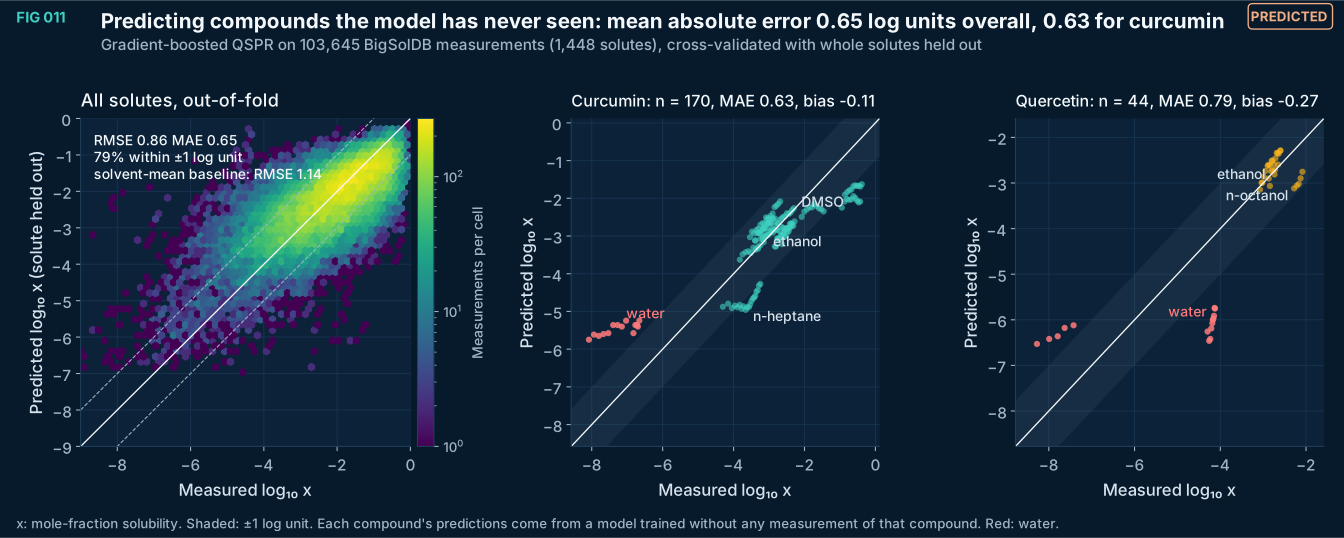
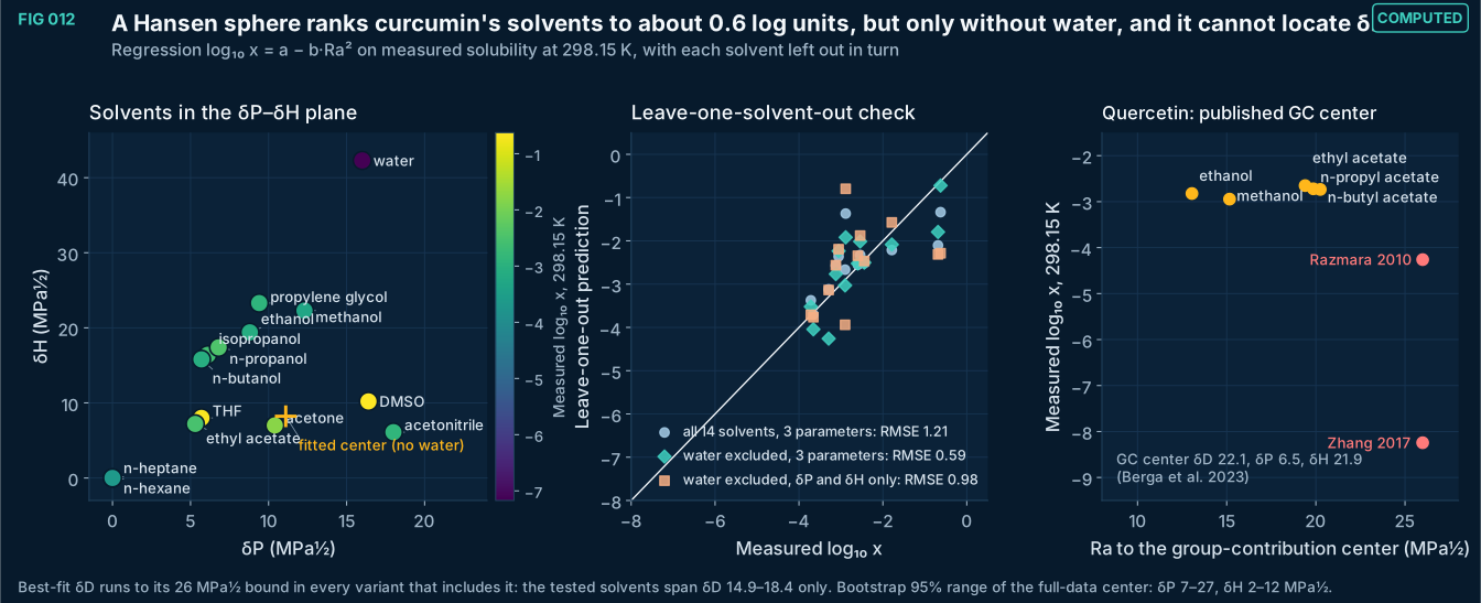
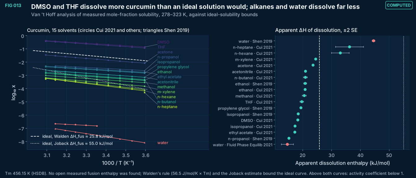
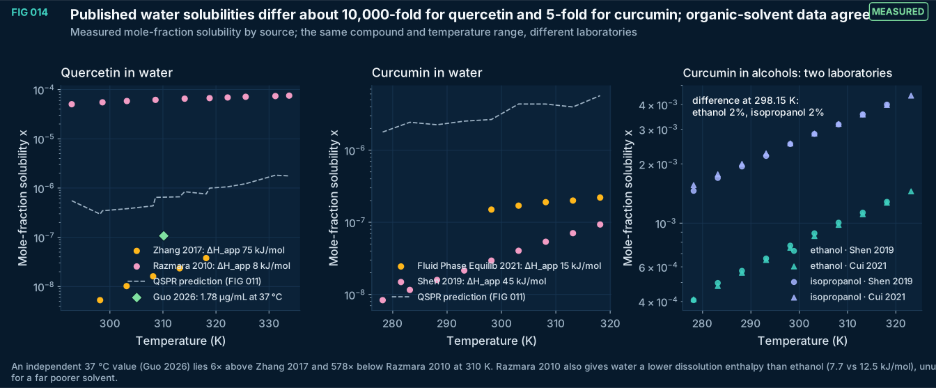
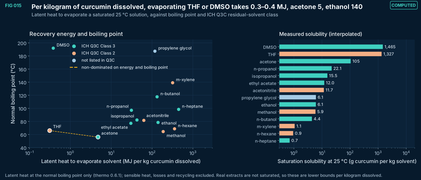
FIG 016–058
Extraction and process
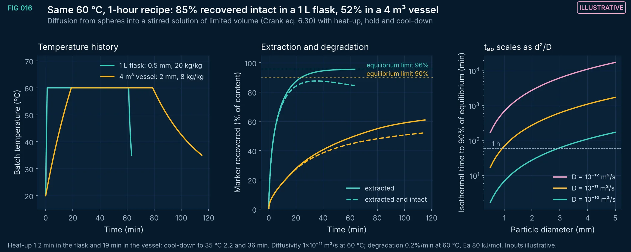
FIG 016Illustrative
An illustrative batch extraction run with an identical temperature and hold time at two scales. Coarser milling (2 mm against 0.5 mm), a lower solvent-to-herb ratio (8 against 20 kg/kg) and slower heat transfer cut the intact recovery from 85% to 52%. Isothermal time to 90% of equilibrium scales with the square of particle diameter over diffusivity.
Method, sources and limits
- Method
- Crank eq. 6.30 with transformed time τ = ∫D(T)dt / r²; D Arrhenius (Ea 20 kJ/mol); first-order degradation (Ea 80 kJ/mol); lumped jacket heat transfer (U = 500 W/m²K, steam 120 °C).
- Sources and code
- Python port of the EUTECNIQ process-engineering page model (src/modules/process/mod.js), verified to reproduce the page's JavaScript output to machine precision for the default case. Crank J. The Mathematics of Diffusion, 2nd ed., Oxford 1975, eq. 6.30 and sec. 7.2. Scripts 04_extraction_and_process/extract_model.py and extract_figs.py.
- Supports
- Why particle size, solvent ratio and heat-up time must be scaled deliberately rather than copied from the laboratory.
- Does not support
- Any yield, time or degradation figure for a real botanical extraction.
- Limitations
- Every input (diffusivity, activation energies, degradation rate, extractable content, heat-transfer coefficient) is illustrative, not measured for any botanical.
- Spherical, uniform particles with partition coefficient 1; no swelling, no matrix binding, no solvent-composition effects.
- Degradation is applied to the whole marker inventory, extracted or not.
Vector (SVG) · Full-size image · data (flask) (CSV) · data (vessel) (CSV)
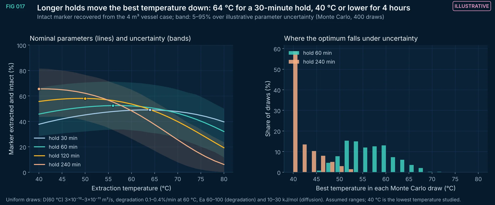
FIG 017Illustrative
Higher temperature speeds diffusion (low activation energy) but accelerates degradation (high activation energy), so intact recovery peaks at an intermediate temperature that falls as the hold lengthens. Under the assumed parameter ranges the location of the optimum is itself uncertain, which is the argument for measuring degradation kinetics before fixing a process temperature.
Method, sources and limits
- Method
- Model of FIG 016 evaluated on a temperature grid; Monte Carlo propagation over four parameters with independent uniform priors (seed 20261105).
- Sources and code
- Python port of the EUTECNIQ process-engineering page model (src/modules/process/mod.js), verified to reproduce the page's JavaScript output to machine precision for the default case. Crank J. The Mathematics of Diffusion, 2nd ed., Oxford 1975, eq. 6.30 and sec. 7.2. Scripts 04_extraction_and_process/extract_model.py and extract_figs.py.
- Supports
- The qualitative trade-off and the value of measuring degradation kinetics early.
- Does not support
- A recommended extraction temperature for any material.
- Limitations
- Every input (diffusivity, activation energies, degradation rate, extractable content, heat-transfer coefficient) is illustrative, not measured for any botanical.
- Spherical, uniform particles with partition coefficient 1; no swelling, no matrix binding, no solvent-composition effects.
- Degradation is applied to the whole marker inventory, extracted or not.
- Parameter ranges are assumptions, not a fitted posterior.
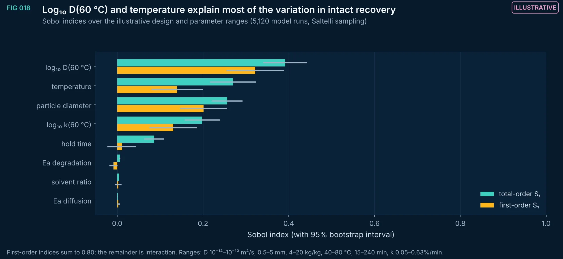
FIG 018Illustrative
Variance-based global sensitivity of intact marker recovery to four design variables and four material parameters. Inputs with large total-order but small first-order indices act mainly through interactions; for example, temperature matters through its coupling with diffusivity and degradation rate.
Method, sources and limits
- Method
- SALib 1.5 Saltelli/Sobol sampling (N = 512, no second-order terms), model of FIG 016 in the 4 m³ vessel.
- Sources and code
- Python port of the EUTECNIQ process-engineering page model (src/modules/process/mod.js), verified to reproduce the page's JavaScript output to machine precision for the default case. Crank J. The Mathematics of Diffusion, 2nd ed., Oxford 1975, eq. 6.30 and sec. 7.2. Scripts 04_extraction_and_process/extract_model.py and extract_figs.py.
- Supports
- Which quantities to measure first when building a real extraction model.
- Does not support
- Sensitivities for any specific plant material.
- Limitations
- Every input (diffusivity, activation energies, degradation rate, extractable content, heat-transfer coefficient) is illustrative, not measured for any botanical.
- Spherical, uniform particles with partition coefficient 1; no swelling, no matrix binding, no solvent-composition effects.
- Degradation is applied to the whole marker inventory, extracted or not.
- Indices depend on the chosen ranges; they rank inputs for this hypothetical problem only.
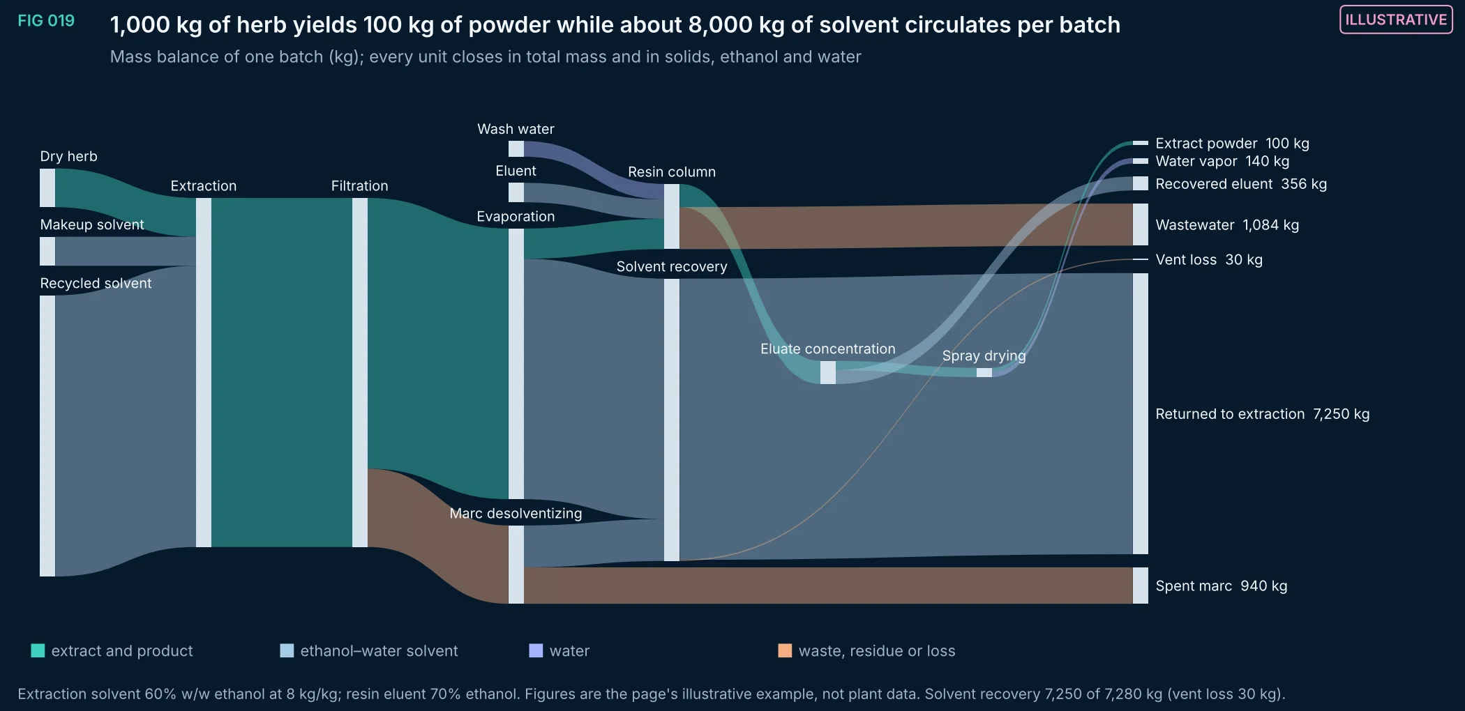
FIG 019Illustrative
Mass flows of an illustrative 1,000 kg batch from dry herb through extraction, filtration, evaporation, resin purification, eluate concentration and spray drying. Solvent circulation dominates the mass moved: about 8,000 kg of 60% ethanol per 100 kg of powder, of which 7,250 kg is recovered and returned. Each unit closes in total mass and in each component (checked in the script).
Method, sources and limits
- Method
- Stream table from the process-engineering page, rendered as a column Sankey; per-unit, per-component balance asserted before plotting.
- Sources and code
- EUTECNIQ process-engineering page, illustrative mass balance (src/modules/process/mod.js, MS_LINKS). Script 04_extraction_and_process/extract_figs.py.
- Supports
- Why solvent recovery dominates equipment sizing and operating cost in ethanol extraction.
- Does not support
- Yields or solvent losses of any real process.
- Limitations
- Illustrative stream values chosen to close; they are not measured or designed for a specific botanical.
- Energy flows are not shown (see FIG 015 and FIG 020).
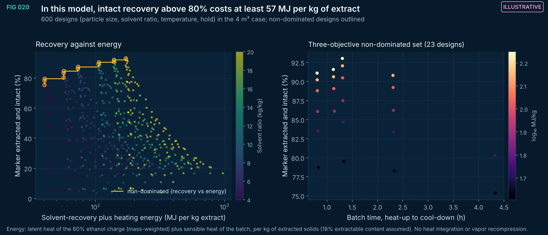
FIG 020Illustrative
A full-factorial sweep of the illustrative extraction model shows the trade-off between intact recovery, energy per kilogram of extract and batch time. High recovery requires fine particles or high solvent ratios; high solvent ratios raise recovery energy roughly in proportion. The non-dominated set is where a real design would be chosen once the inputs are measured.
Method, sources and limits
- Method
- Model of FIG 016; 5 × 6 × 5 × 4 factorial; Pareto filtering on (−recovery, energy) and (−recovery, energy, batch time).
- Sources and code
- Python port of the EUTECNIQ process-engineering page model (src/modules/process/mod.js), verified to reproduce the page's JavaScript output to machine precision for the default case. Crank J. The Mathematics of Diffusion, 2nd ed., Oxford 1975, eq. 6.30 and sec. 7.2. Scripts 04_extraction_and_process/extract_model.py and extract_figs.py.
- Supports
- How a design trade-off would be framed and which inputs set it.
- Does not support
- Energy or cost figures for an actual plant.
- Limitations
- Every input (diffusivity, activation energies, degradation rate, extractable content, heat-transfer coefficient) is illustrative, not measured for any botanical.
- Spherical, uniform particles with partition coefficient 1; no swelling, no matrix binding, no solvent-composition effects.
- Degradation is applied to the whole marker inventory, extracted or not.
- Energy accounting is simplified (no recovery losses, no heat integration).
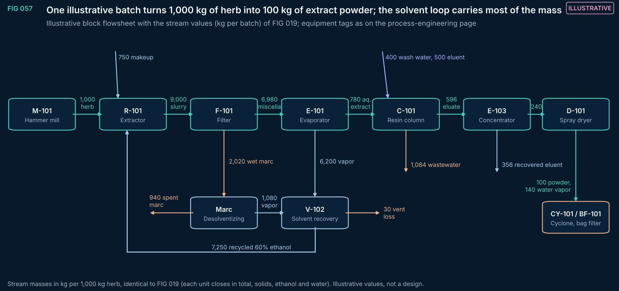
FIG 057Illustrative
Block flowsheet of the illustrative botanical extraction train with per-batch stream masses: milling, ethanol–water extraction, filtration, evaporation, adsorbent-resin purification, eluate concentration and spray drying, with marc desolventizing and a solvent-recovery loop that returns 7,250 kg of the 8,000 kg extraction charge.
Method, sources and limits
- Method
- Block diagram drawn from the stream table of FIG 019.
- Sources and code
- EUTECNIQ process-engineering page, illustrative 1,000 kg batch (src/modules/process/mod.js, MS_LINKS; equipment tags as on the page). Script 04_extraction_and_process/process_figs.py.
- Supports
- The structure of an integrated extraction-to-powder train.
- Does not support
- Equipment selection or capacity claims.
- Limitations
- Illustrative process; no specific botanical, equipment size or regulatory filing is implied.
- Utilities and controls are not shown.
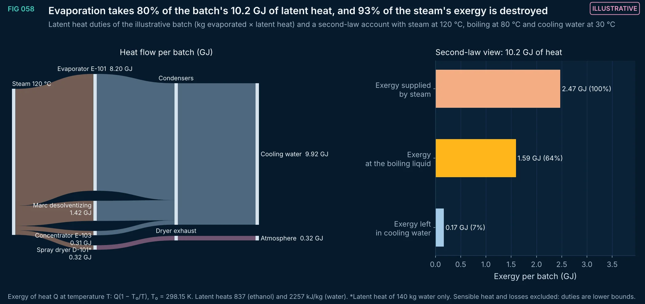
FIG 058Illustrative
Latent heat needed to evaporate the solvent and water streams of the illustrative batch, and where it goes. The 10.2 GJ supplied as steam ends almost entirely in cooling water; in second-law terms, 2.47 GJ of exergy is supplied and only 0.17 GJ remains in the cooling water. This is the quantitative case for heat integration or mechanical vapor recompression in an ethanol extraction plant.
Method, sources and limits
- Method
- Q = Σ m·Δh_vap per unit from the stream table (FIG 019); exergy of heat by the Carnot factor at the stated temperatures.
- Sources and code
- EUTECNIQ process-engineering page, illustrative 1,000 kg batch (src/modules/process/mod.js, MS_LINKS; equipment tags as on the page). Script 04_extraction_and_process/process_figs.py.
- Supports
- Why energy recovery is a design priority for solvent-based extraction.
- Does not support
- Energy consumption figures for any real plant.
- Limitations
- Constant latent heats and an assumed single boiling temperature (80 °C) for all evaporations; vacuum operation would lower it.
- Spray-dryer duty is the latent heat of 140 kg water only; real dryers need several times more because of air heating.
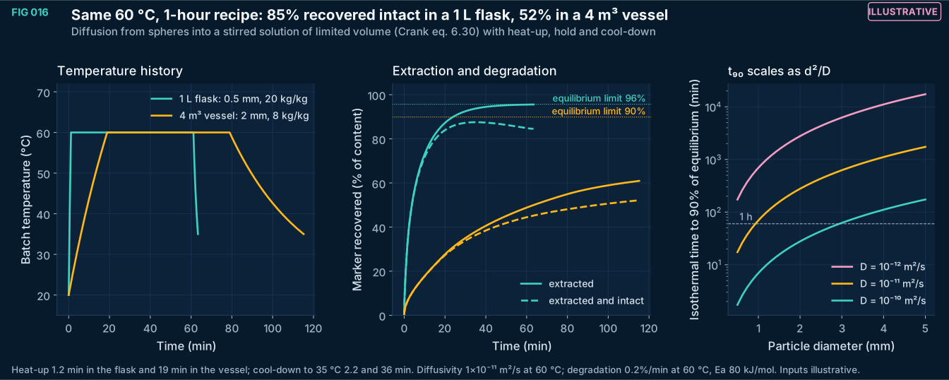
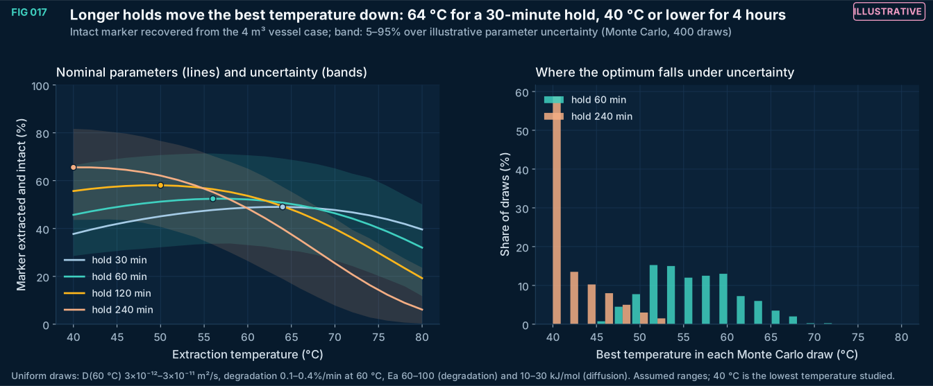
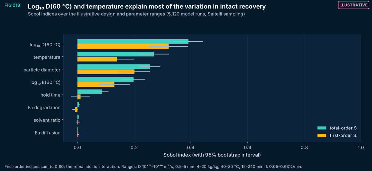
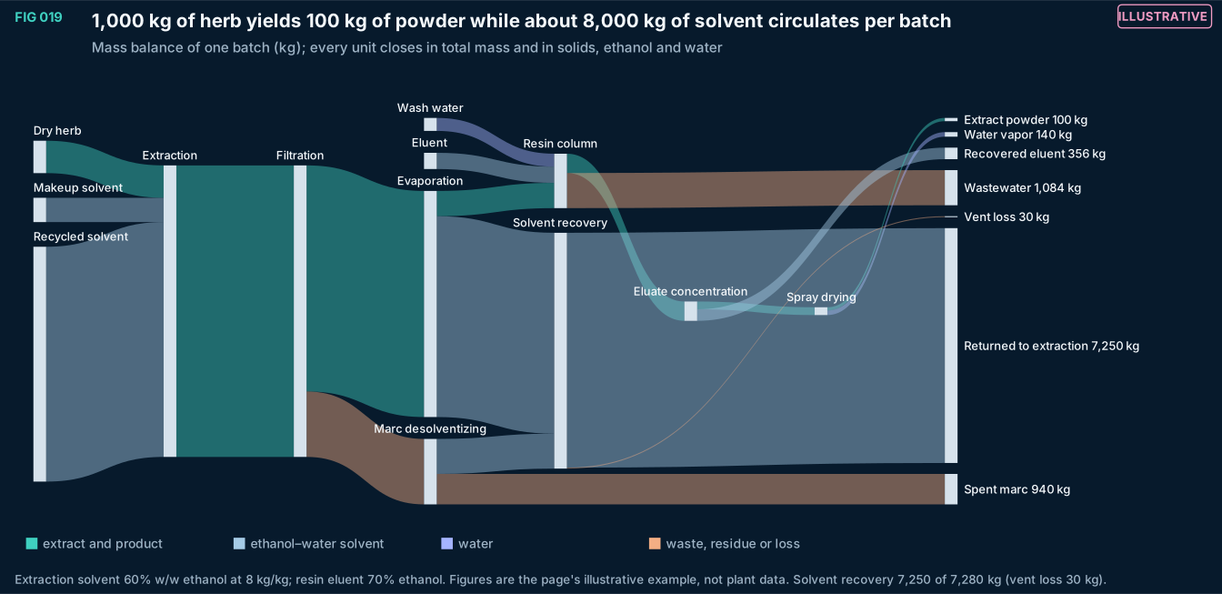
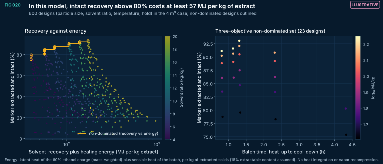
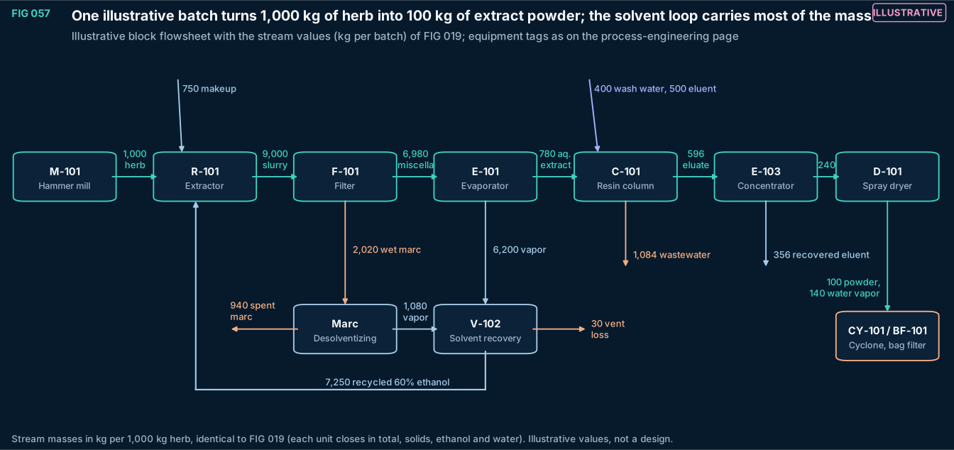
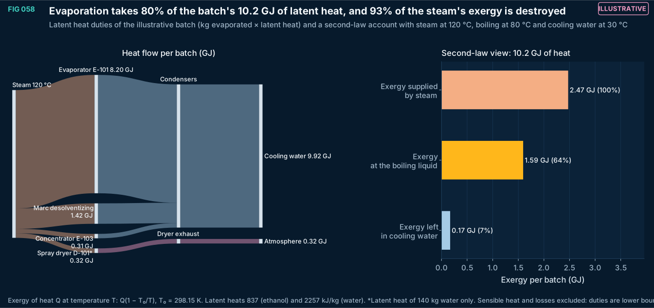
FIG 021–051
Formulation and stability
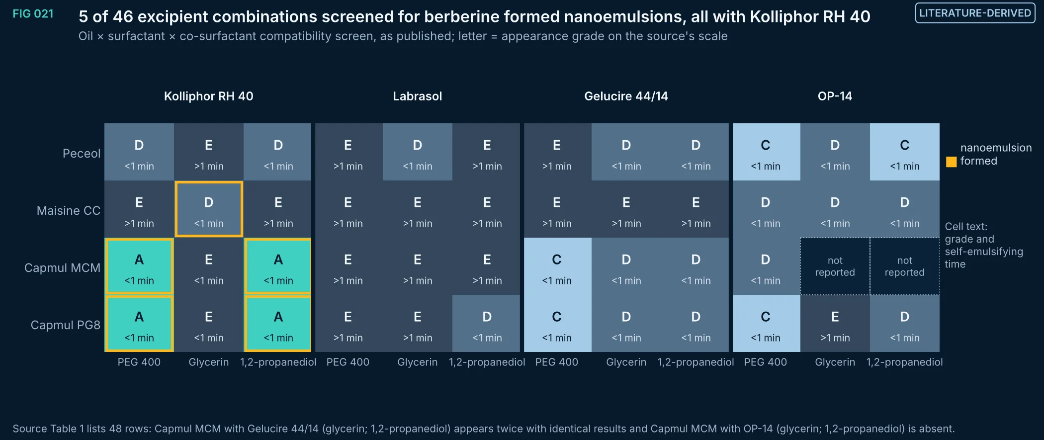
FIG 021Literature-derived
Excipient compatibility screen for berberine hydrochloride SMEDDS (Chen et al. 2024, Table 1). Only combinations with Kolliphor RH 40 formed nanoemulsions; the authors' final formulation was Capmul MCM 55%, Kolliphor RH 40 22.5% and 1,2-propanediol 22.5% (w/w). Two rows of the published table are duplicates and two combinations are missing.
Method, sources and limits
- Method
- Published table re-plotted without modification; duplicates detected programmatically.
- Sources and code
- Chen X et al. Self-microemulsifying drug delivery system to enhance oral bioavailability of berberine hydrochloride in rats. Pharmaceutics 2024;16(9):1116. doi:10.3390/pharmaceutics16091116. PMID 39339154, PMC11435259 Script 05_delivery_QbD/form_figs.py; transcriptions in form_data.py; source XML in 00_provenance/literature.
- Supports
- Kolliphor RH 40 as the decisive excipient in this screen.
- Does not support
- Generalization to other berberine salts, doses or excipient grades.
- Limitations
- Visual grading on the source's scale; the grading definitions are those of the source.
- Single laboratory, blank (drug-free) and drug-loaded behavior can differ.
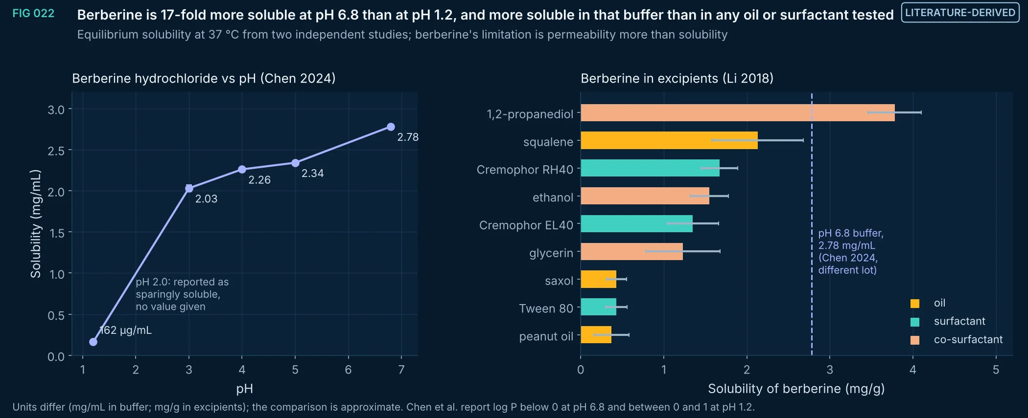
FIG 022Literature-derived
Berberine hydrochloride solubility rises from 0.162 mg/mL at pH 1.2 to 2.78 mg/mL at pH 6.8 (Chen et al. 2024); in three oils and three surfactants it stays at or below 2.13 mg/g, and only 1,2-propanediol (3.78 mg/g) exceeds the pH 6.8 buffer value (Li et al. 2018). For a hydrophilic quaternary cation, lipid systems act mainly on permeability and transport, not on dissolution.
Method, sources and limits
- Method
- Published values re-plotted; no fitting.
- Sources and code
- Chen X et al. Self-microemulsifying drug delivery system to enhance oral bioavailability of berberine hydrochloride in rats. Pharmaceutics 2024;16(9):1116. doi:10.3390/pharmaceutics16091116. PMID 39339154, PMC11435259 Li J et al. Self-nanoemulsifying system improves oral absorption and enhances anti-acute myeloid leukemia activity of berberine. J Nanobiotechnology 2018;16:76. doi:10.1186/s12951-018-0402-x. PMID 30290822, PMC6172716 Script 05_delivery_QbD/form_figs.py; transcriptions in form_data.py; source XML in 00_provenance/literature.
- Supports
- Framing berberine as a permeability-limited rather than solubility-limited problem in intestinal conditions.
- Does not support
- Claims about absorption mechanisms of any formulation.
- Limitations
- Two laboratories, different material lots and media; mg/mL and mg/g are not interchangeable without densities.
- Gastric solubility at pH 2.0 was not reported numerically.
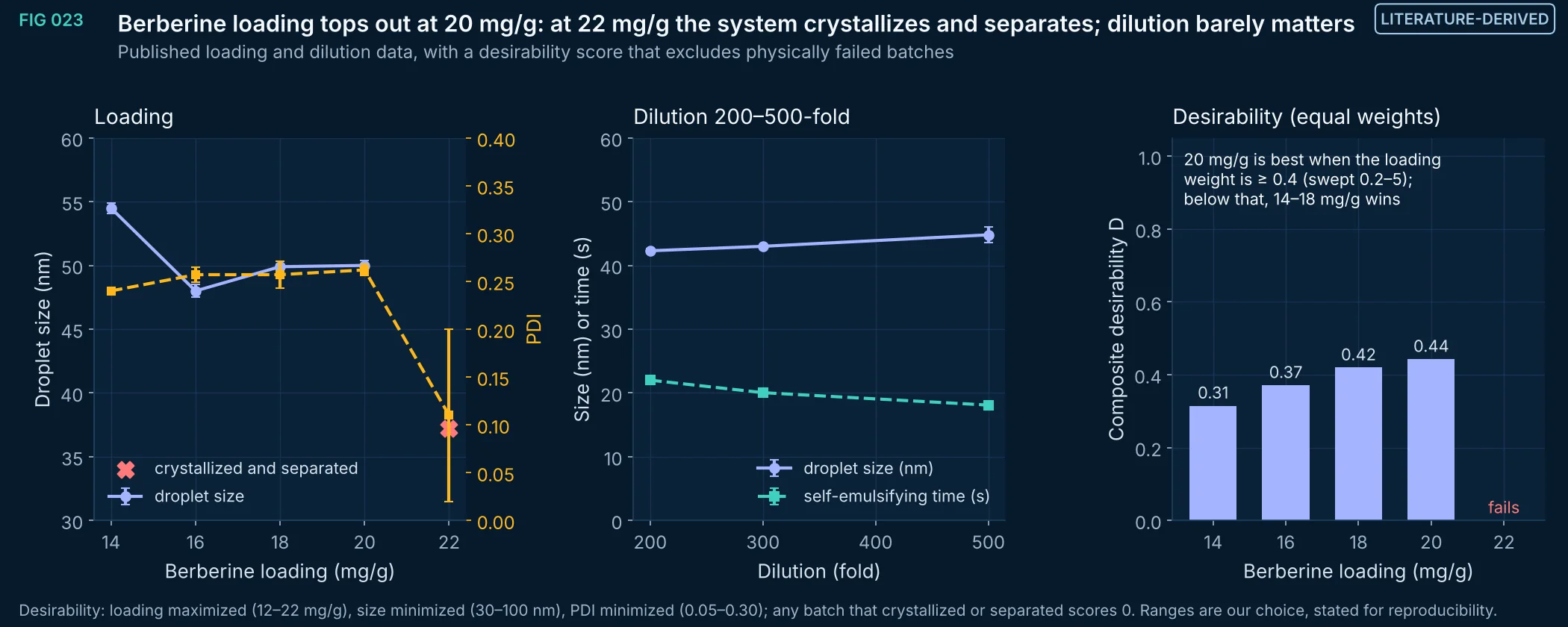
FIG 023Literature-derived
Droplet size and polydispersity of berberine SMEDDS at 14–22 mg/g drug and after 200–500-fold dilution (Chen et al. 2024, Tables 2 and 3). At 22 mg/g the system crystallized and separated on centrifugation; its smaller droplet size does not make it a better batch. A Derringer desirability score with a feasibility gate picks 20 mg/g, the loading the authors used, with equal weights; with loading weighted at 0.3 or less relative to size and PDI, 14–18 mg/g scores higher.
Method, sources and limits
- Method
- Published means ± SD re-plotted; Derringer–Suich desirability (geometric mean of one-sided linear desirabilities) with a hard feasibility constraint; weight sweep on the loading term.
- Sources and code
- Chen X et al. Self-microemulsifying drug delivery system to enhance oral bioavailability of berberine hydrochloride in rats. Pharmaceutics 2024;16(9):1116. doi:10.3390/pharmaceutics16091116. PMID 39339154, PMC11435259 Script 05_delivery_QbD/form_figs.py; transcriptions in form_data.py; source XML in 00_provenance/literature.
- Supports
- Treating physical stability as a constraint rather than one more response to average.
- Does not support
- Long-term stability or in vivo performance at any loading.
- Limitations
- Five loadings and three dilutions, n = 3 each; no replicate batches.
- Desirability ranges are analyst choices.
Vector (SVG) · Full-size image · data (dilution) (CSV) · data (loading) (CSV)
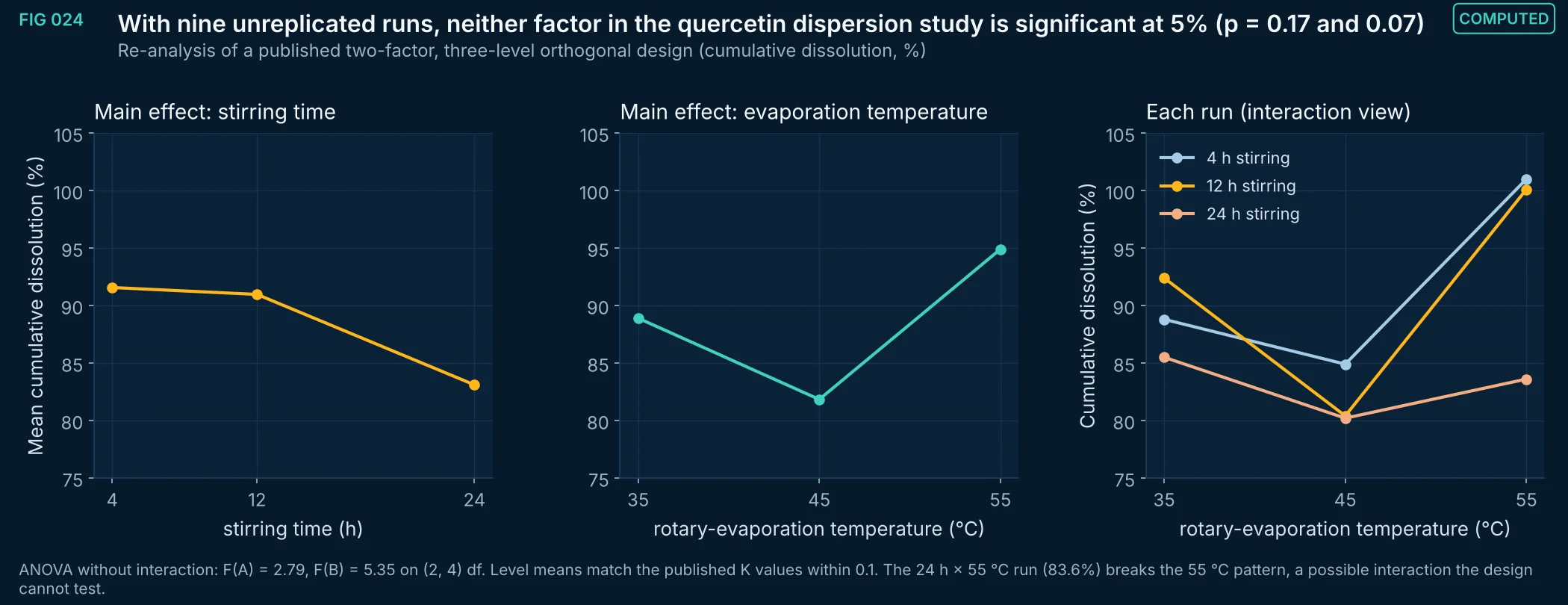
FIG 024Computed
Main-effect and run-level plots for the published L9-type design (stirring time × rotary-evaporation temperature) of quercetin solid dispersions. The authors ranked factors by range (8.5 and 6.0 points). A two-way ANOVA on the same nine values gives p = 0.17 for stirring time and p = 0.07 for temperature, so the ranking is not supported statistically; the 4 h, 55 °C condition is a reasonable choice but not a demonstrated optimum.
Method, sources and limits
- Method
- Two-way additive ANOVA (residual df 4) on the published responses; level means compared with the published K values.
- Sources and code
- Guo et al. Formulation development and characterization of quercetin solid dispersions with integrated in vitro release and in vivo pharmacokinetic assessment. Pharmaceuticals 2026;19(10):1625. doi:10.3390/ph19101625. PMID 42943322, PMC13708282 Script 05_delivery_QbD/form_figs.py; transcriptions in form_data.py; source XML in 00_provenance/literature.
- Supports
- Replicated or response-surface designs before claiming an optimum.
- Does not support
- Any conclusion that either factor has no effect.
- Limitations
- No replicates: interaction and pure error are confounded in the residual.
- Responses are single cumulative-dissolution values at one time point.
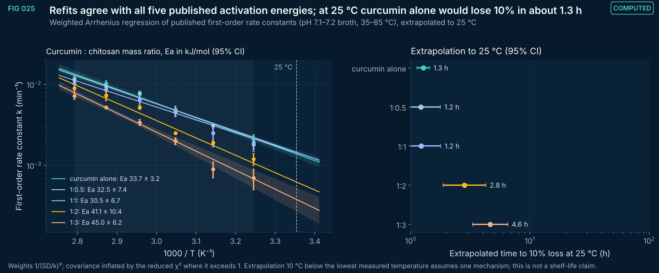
FIG 025Computed
First-order degradation rate constants of curcumin (10 µg/mL) in cation-adjusted Mueller–Hinton broth at pH 7.1–7.2, alone and with chitosan (Dechayont et al. 2026, Table 2), refitted by weighted Arrhenius regression. Every published activation energy lies inside the 95% interval of the refit. Extrapolation to 25 °C gives the time to 10% loss with its 95% interval; higher chitosan ratios lengthen it.
Method, sources and limits
- Method
- Weighted least squares of ln k on 1/T; delta-method intervals for ln k at 25 °C; t₉₀ = ln(10/9)/k.
- Sources and code
- Dechayont B, Brunaugh AD. Chitosan stabilizes curcumin against hydrolysis and potentiates antimicrobial activity against Pseudomonas aeruginosa in a pH-dependent manner. ACS Omega 2026;11(31):46088–46104. doi:10.1021/acsomega.6c02415. PMID 42597930, PMC13470882 Script 05_delivery_QbD/form_figs.py; transcriptions in form_data.py; source XML in 00_provenance/literature.
- Supports
- Using Arrhenius kinetics to plan accelerated stability work for curcumin systems.
- Does not support
- A shelf life for any product.
- Limitations
- Rate constants are for a microbiological broth with 1% DMSO, not a formulation or food matrix.
- UV 420 nm assay measures loss of the chromophore, not identity of products.
- Extrapolation below 35 °C is outside the measured range.
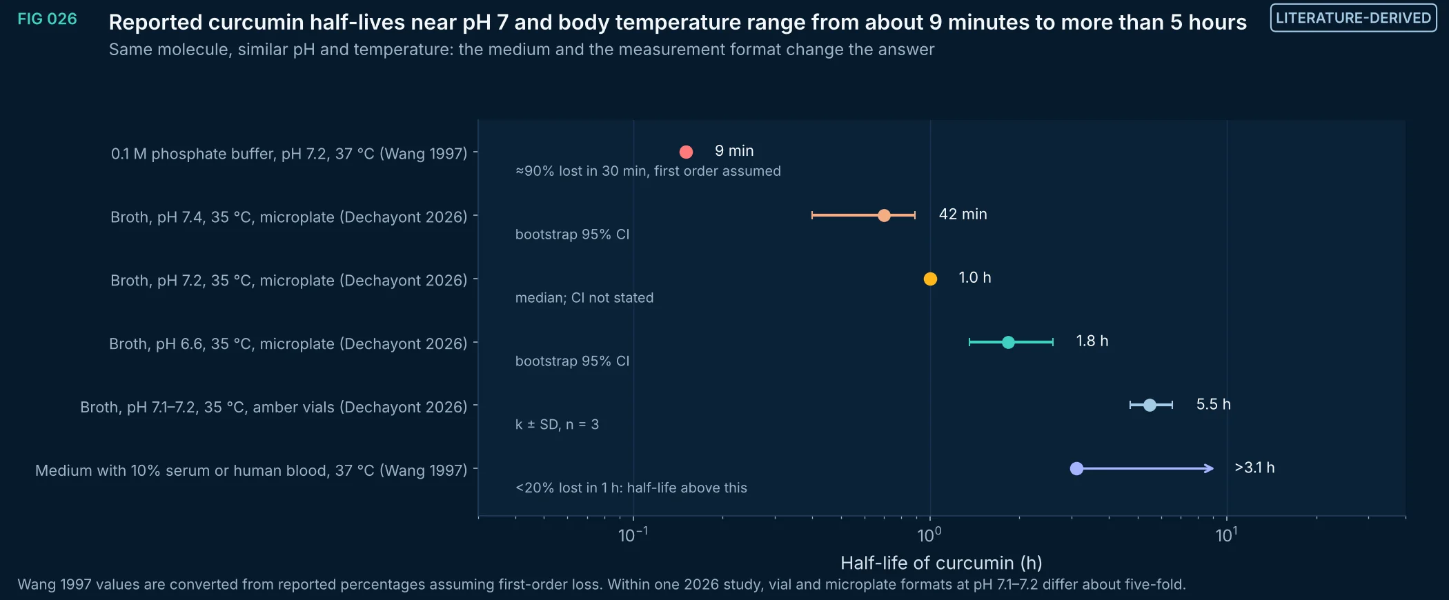
FIG 026Literature-derived
Half-lives of curcumin reported or derived for near-neutral pH at 35–37 °C. Phosphate buffer gives minutes; protein-containing broth gives hours, and the same broth gives different values in amber vials and in microplates. A stability number for curcumin is meaningful only with its medium, container, concentration and assay.
Method, sources and limits
- Method
- Published half-lives and rate constants; percentages converted with t½ = ln 2 / k for first-order loss.
- Sources and code
- Dechayont B, Brunaugh AD. Chitosan stabilizes curcumin against hydrolysis and potentiates antimicrobial activity against Pseudomonas aeruginosa in a pH-dependent manner. ACS Omega 2026;11(31):46088–46104. doi:10.1021/acsomega.6c02415. PMID 42597930, PMC13470882 Wang YJ et al. Stability of curcumin in buffer solutions and characterization of its degradation products. J Pharm Biomed Anal 1997;15(12):1867-76. PMID 9278892 Script 05_delivery_QbD/form_figs.py; transcriptions in form_data.py; source XML in 00_provenance/literature.
- Supports
- Specifying matrix and method for every stability claim.
- Does not support
- A single 'half-life of curcumin'.
- Limitations
- Different curcumin concentrations, co-solvents, light protection and assays.
- Wang 1997 values are taken from the published abstract (about 90% decomposed within 30 min in 0.1 M phosphate buffer, pH 7.2, 37 °C; about 50% remaining after 8 h in medium with 10% fetal calf serum); the full text was not re-examined.
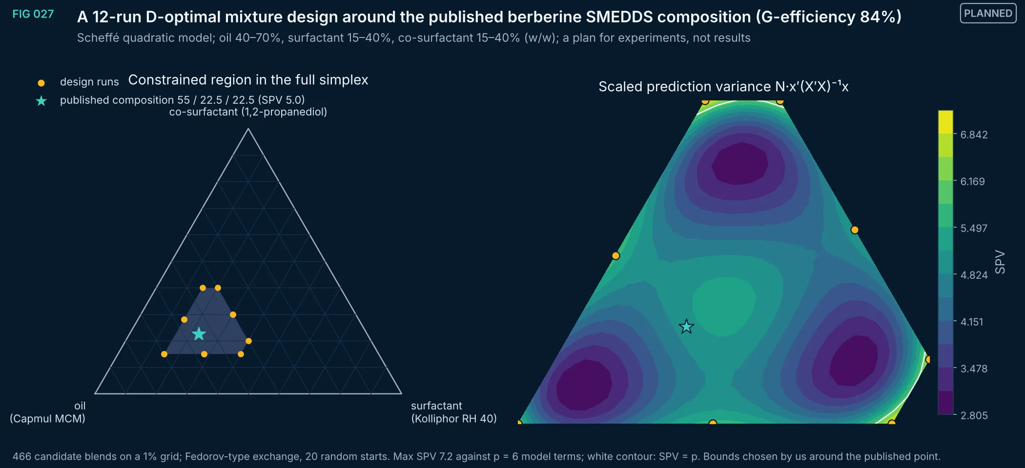
FIG 027Planned
A D-optimal 12-run design for a Scheffé quadratic mixture model in the oil–surfactant–co-surfactant region around the published berberine SMEDDS composition. Scaled prediction variance stays at or below 7.2 across the region (G-efficiency 84%), and is 5.0 at the published point. This is a plan for measuring droplet size, emulsification time and drug loading, not a result.
Method, sources and limits
- Method
- Candidate set on a 1% grid within bounds; exchange algorithm maximizing log det(X′X) for the 6-term Scheffé quadratic; prediction variance evaluated on all candidates.
- Sources and code
- Published composition: Chen X et al. Self-microemulsifying drug delivery system to enhance oral bioavailability of berberine hydrochloride in rats. Pharmaceutics 2024;16(9):1116. doi:10.3390/pharmaceutics16091116. PMID 39339154, PMC11435259 Bounds are analyst assumptions. Script 05_delivery_QbD/form_figs.py; transcriptions in form_data.py; source XML in 00_provenance/literature.
- Supports
- An efficient experiment to map the SMEDDS region rather than one-factor-at-a-time testing.
- Does not support
- Any predicted droplet size or stability.
- Limitations
- No responses exist for these blends; the design only guarantees how well a quadratic model could be estimated.
- Bounds and model order are assumptions; a special-cubic term may be needed.
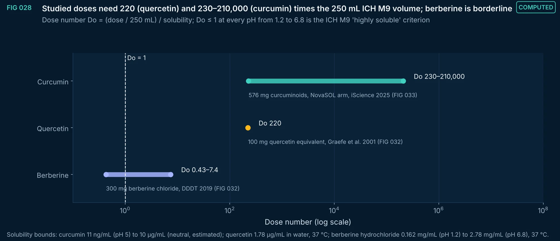
FIG 028Computed
Dose numbers for the main doses in the human studies cited in this note (curcumin about 570 mg, quercetin 100 mg, berberine chloride 300 mg); higher curcumin doses in the cited studies (2.28 g; 10–12 g) give proportionally larger values. Berberine chloride at 300 mg exceeds Do = 1 at pH 1.2 but not at pH 6.8; quercetin and curcumin exceed it by two to five orders of magnitude, so formulation can change dissolution but cannot make these doses dissolve in gastrointestinal volumes as free molecules.
Method, sources and limits
- Method
- Do = (D/250 mL)/Cs (ICH M9 volume); bounds from the lowest and highest solubility values cited.
- Sources and code
- 11 ng/mL at pH 5 (Brotons-Canto et al. Pharmaceutics 2021;13:361, quoting Tønnesen et al. 2002); 1–10 µg/mL estimated at neutral pH (Nelson et al. J Med Chem 2017); 1.78 ± 0.17 µg/mL in water at 37 °C (Guo et al. 2026); berberine hydrochloride 0.162 mg/mL at pH 1.2 to 2.78 mg/mL at pH 6.8, 37 °C (Chen et al. 2024). ICH M9 (2019) Biopharmaceutics Classification System-based biowaivers. Script 05_delivery_QbD/form_figs.py; transcriptions in form_data.py; source XML in 00_provenance/literature.
- Supports
- Why curcumin and quercetin need solubilizing or supersaturating formulations.
- Does not support
- A BCS classification for any product.
- Limitations
- Solubility values come from different laboratories, temperatures and media; biorelevant media with bile salts raise solubility of lipophilic compounds.
- Dose number ignores permeability and metabolism.
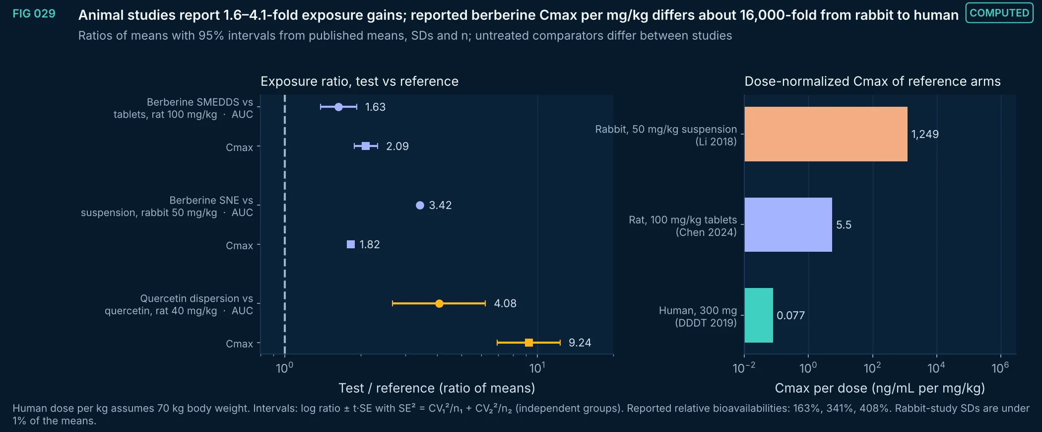
FIG 029Computed
Exposure ratios of formulated against reference arms in three animal studies (two berberine, one quercetin), with 95% intervals reconstructed from the published summary statistics, and the dose-normalized peak concentration of each berberine study's reference arm. Per mg/kg, the rat reference arm reports about 71 times and the rabbit arm about 16,000 times the human peak concentration, which signals large differences in species, dose, assay or analyte; fold changes from one model do not transfer to people.
Method, sources and limits
- Method
- Ratio of means with log-normal delta-method interval (t with n₁+n₂−2 df); dose normalization by mg/kg.
- Sources and code
- Chen X et al. Self-microemulsifying drug delivery system to enhance oral bioavailability of berberine hydrochloride in rats. Pharmaceutics 2024;16(9):1116. doi:10.3390/pharmaceutics16091116. PMID 39339154, PMC11435259 Li J et al. Self-nanoemulsifying system improves oral absorption and enhances anti-acute myeloid leukemia activity of berberine. J Nanobiotechnology 2018;16:76. doi:10.1186/s12951-018-0402-x. PMID 30290822, PMC6172716 Guo et al. Formulation development and characterization of quercetin solid dispersions with integrated in vitro release and in vivo pharmacokinetic assessment. Pharmaceuticals 2026;19(10):1625. doi:10.3390/ph19101625. PMID 42943322, PMC13708282 Human berberine: DDDT 2019;13:129 (FIG 032). Script 05_delivery_QbD/form_figs.py; transcriptions in form_data.py; source XML in 00_provenance/literature.
- Supports
- Treating animal fold changes as hypothesis-generating; the need for human data on any formulation claim.
- Does not support
- Any human bioavailability claim for these formulations.
- Limitations
- Summary statistics only; individual data unavailable.
- Different comparators (tablets, suspension, unformulated powder) and assays (HPLC-UV vs UPLC-MS/MS).
- Human body weight assumed.
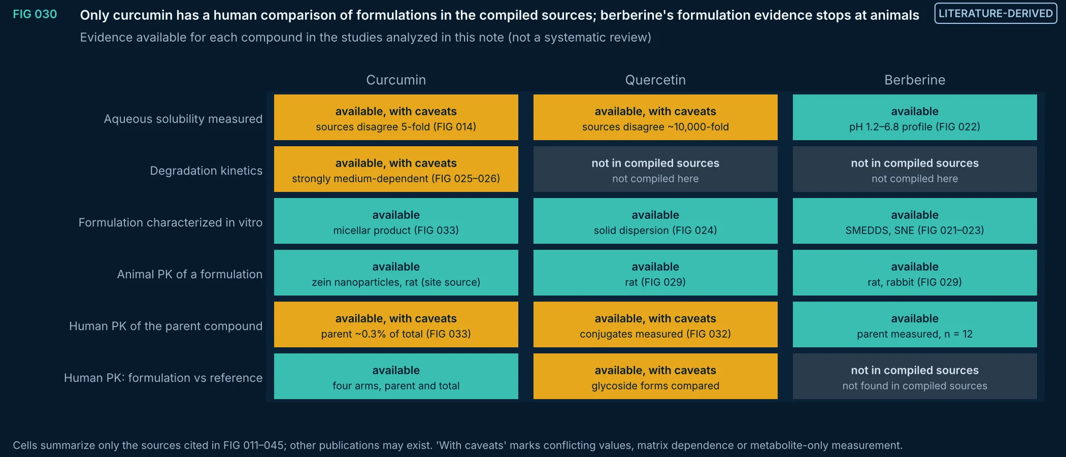
FIG 030Literature-derived
What the studies analyzed in this note do and do not show for each compound. Curcumin has a four-arm human study comparing formulations by unconjugated and total curcumin; quercetin's human data compare glycoside forms by conjugate levels; berberine has human data for the parent compound only, and its formulation data are in vitro and in animals.
Method, sources and limits
- Method
- Structured summary of the cited sources; categories defined before filling the table.
- Sources and code
- Sources as cited in FIG 011–045 and their metadata files. Script 05_delivery_QbD/form_figs.py; transcriptions in form_data.py; source XML in 00_provenance/literature.
- Supports
- Prioritizing human pharmacokinetic studies for berberine formulations.
- Does not support
- Any claim that a study does not exist.
- Limitations
- Not a systematic review; absence here means absence from the compiled sources only.
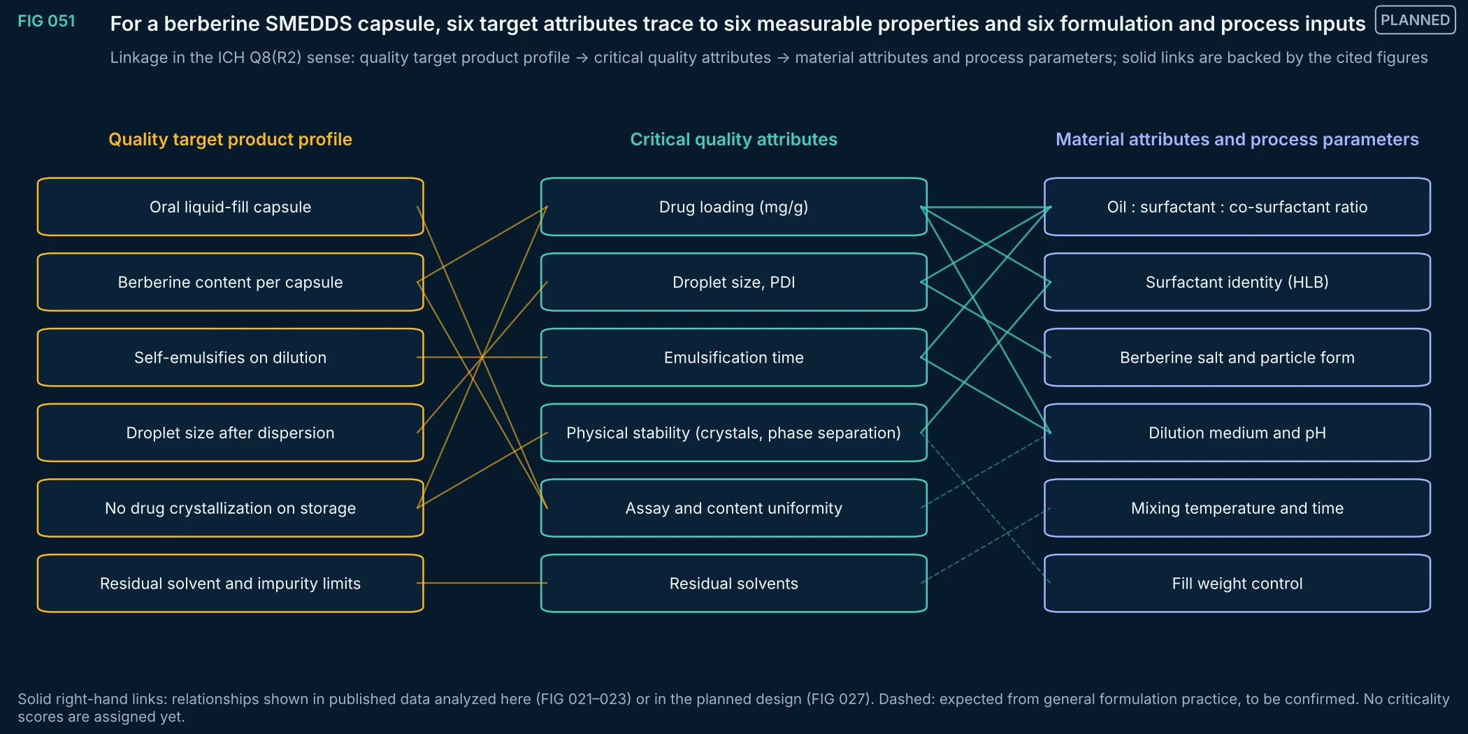
FIG 051Planned
A first linkage map for a berberine self-microemulsifying capsule, following the ICH Q8(R2) structure: what the product must do, the measurable attributes that express it, and the formulation and process inputs that control them. Links supported by the published data analyzed in this note are drawn solid; others are hypotheses to test.
Method, sources and limits
- Method
- Structured mapping; evidence links taken from FIG 021–023 and FIG 027.
- Sources and code
- ICH Q8(R2) Pharmaceutical Development (2009); ICH Q9(R1) Quality Risk Management (2023). Data sources as in FIG 021–023. Script 04_extraction_and_process/process_figs.py.
- Supports
- How development experiments would be prioritized.
- Does not support
- Any regulatory or product claim.
- Limitations
- Not a risk assessment: no severity, occurrence or detectability scores.
- Product concept only; no EUTECNIQ product of this kind exists.
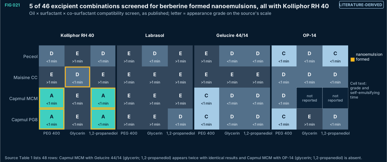
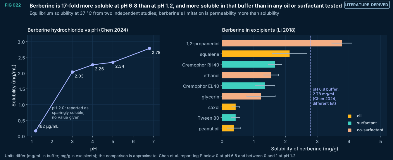
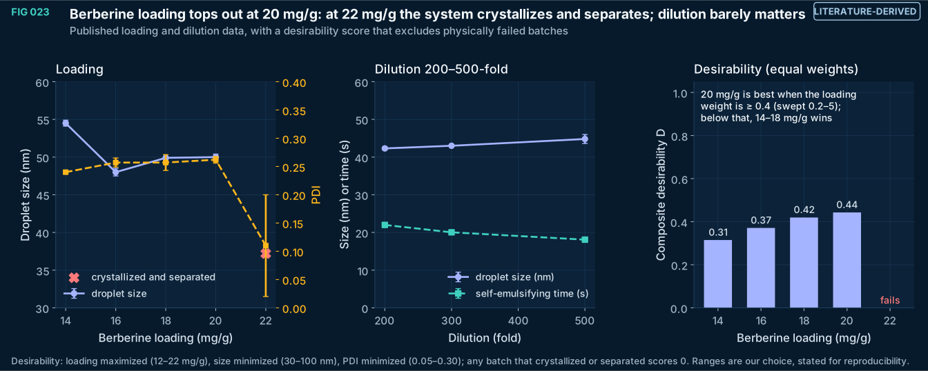
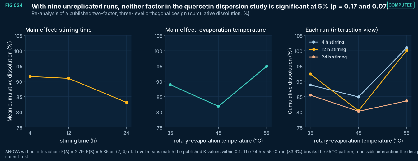
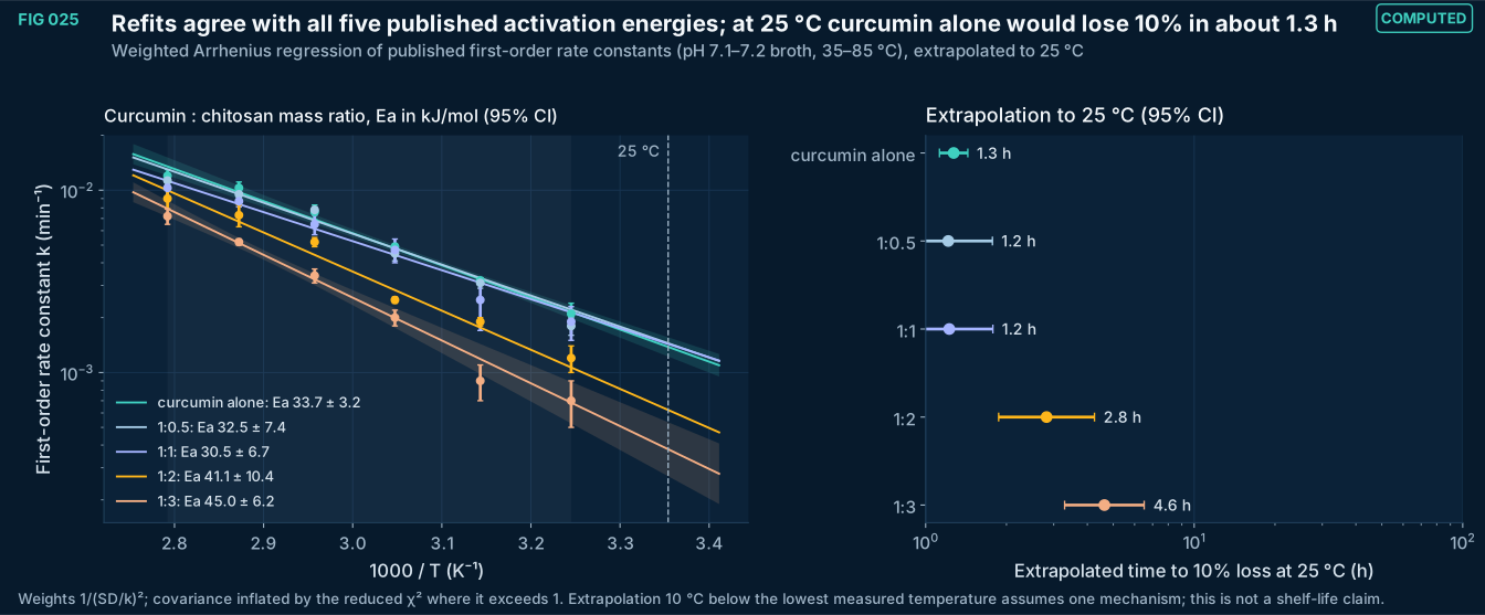
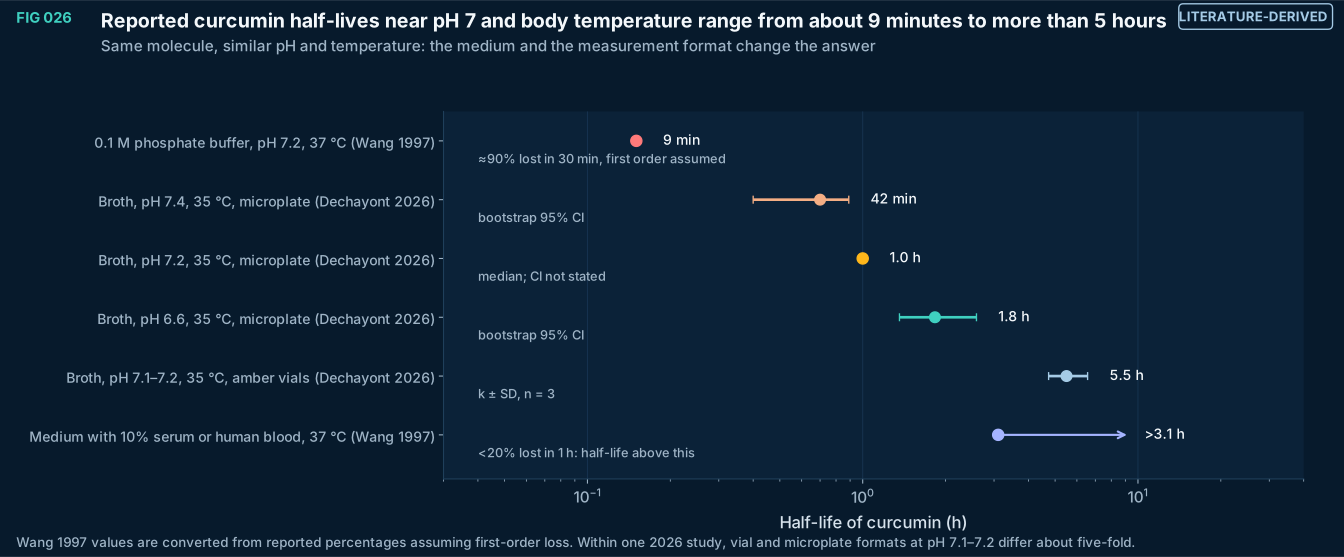
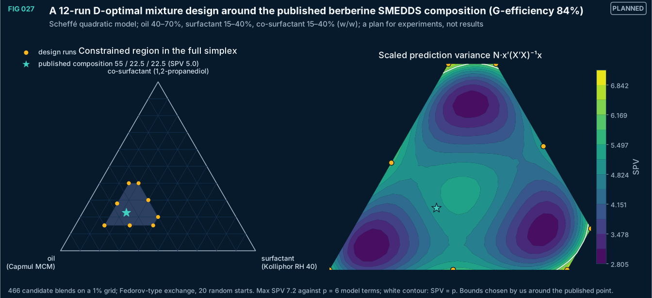
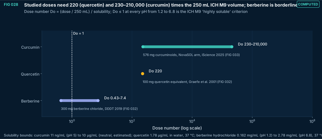
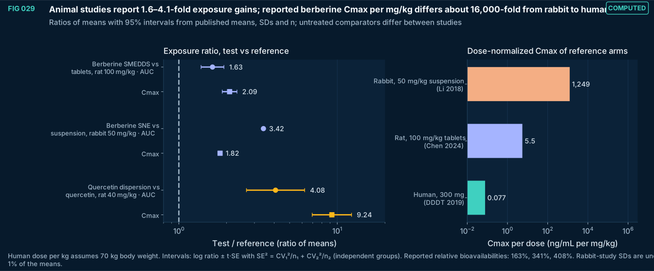
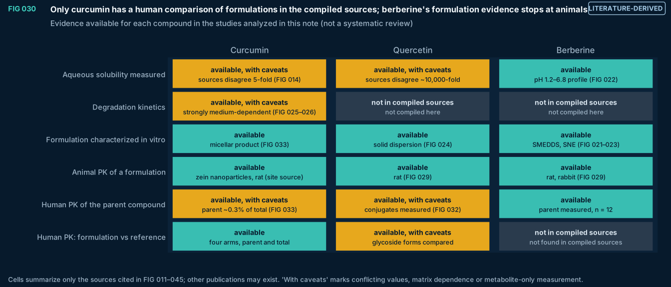
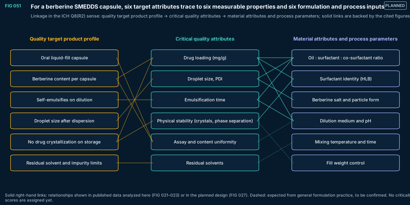
FIG 031–040
Pharmacokinetics
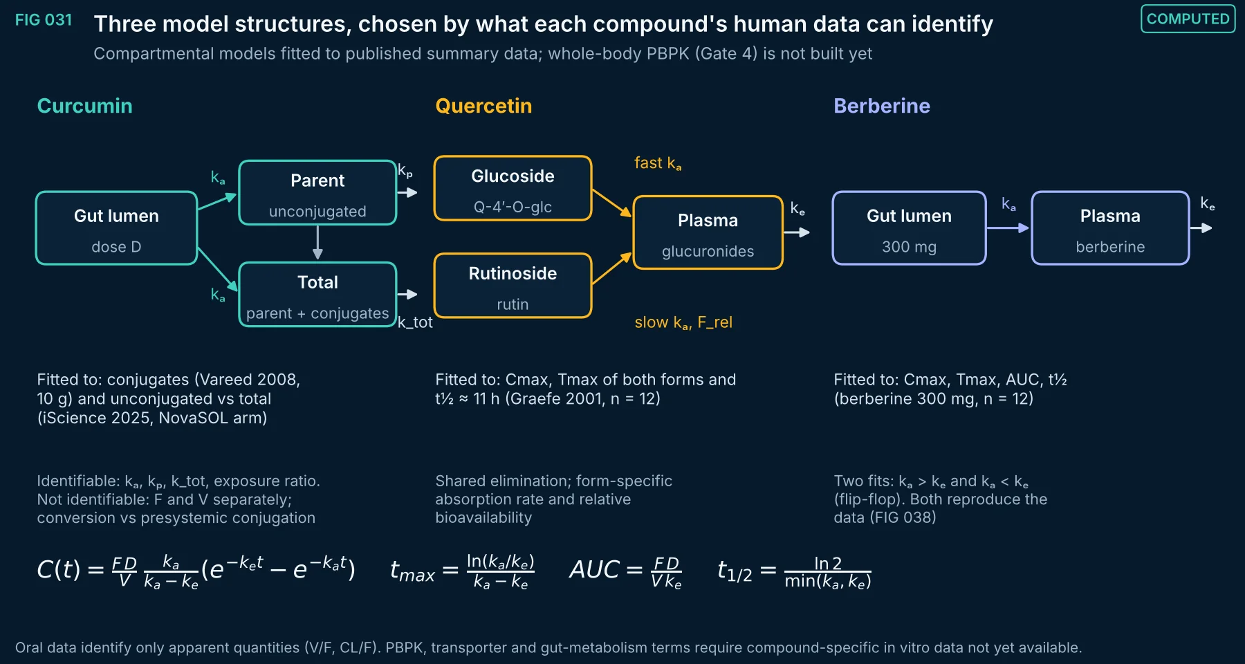
FIG 031Computed
Model structures used for the three compounds, with the equations solved and what each dataset can and cannot identify.
Method, sources and limits
- Method
- Analytic one-compartment oral (Bateman) models; curcumin parent and total curves share the absorption rate.
- Sources and code
- Data: Vareed et al., Cancer Epidemiol Biomarkers Prev 2008;17:1411–1417; iScience 2025;28:112575.; Data: Graefe et al., J Clin Pharmacol 2001;41:492–499 (n = 12 crossover).; Data: Li G, Zhao M, Qiu F, Sun Y, Zhao L. Pharmacokinetic interactions and tolerability of berberine chloride with simvastatin and fenofibrate: an open-label, randomized, parallel study in healthy Chinese subjects. Drug Des Devel Ther 2019;13:129–139. doi:10.2147/DDDT.S185487 (berberine 300 mg single dose, n = 12, Table 6).
- Supports
- Does not support
- Limitations
- Not PBPK. No physiology, transporter or enzyme kinetics are represented.
- Summary-level calibration (no individual data).
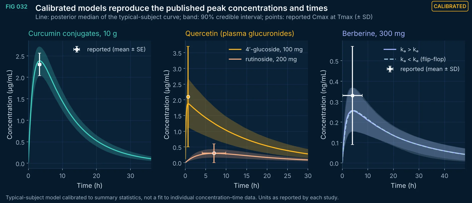
FIG 032Calibrated
Posterior median and 90% interval of the typical-subject concentration–time curve for each dataset, with the reported Cmax and Tmax.
Method, sources and limits
- Method
- PyMC 6.4 NUTS, 4 chains × 2,000 draws after 2,000 tuning steps; likelihood on reported summary statistics (SE = SD/√n).
- Sources and code
- Data: Vareed et al., Cancer Epidemiol Biomarkers Prev 2008;17:1411–1417; iScience 2025;28:112575.; Data: Graefe et al., J Clin Pharmacol 2001;41:492–499 (n = 12 crossover).; Data: Li G, Zhao M, Qiu F, Sun Y, Zhao L. Pharmacokinetic interactions and tolerability of berberine chloride with simvastatin and fenofibrate: an open-label, randomized, parallel study in healthy Chinese subjects. Drug Des Devel Ther 2019;13:129–139. doi:10.2147/DDDT.S185487 (berberine 300 mg single dose, n = 12, Table 6).
- Supports
- The model structures can reproduce the reported summary statistics.
- Does not support
- Any claim about individual subjects or untested formulations.
- Limitations
- Reported means of individual Cmax and Tmax are not the Cmax and Tmax of a mean curve (Jensen gap).
- Quercetin values are plasma glucuronides; no free quercetin was detected in that study.
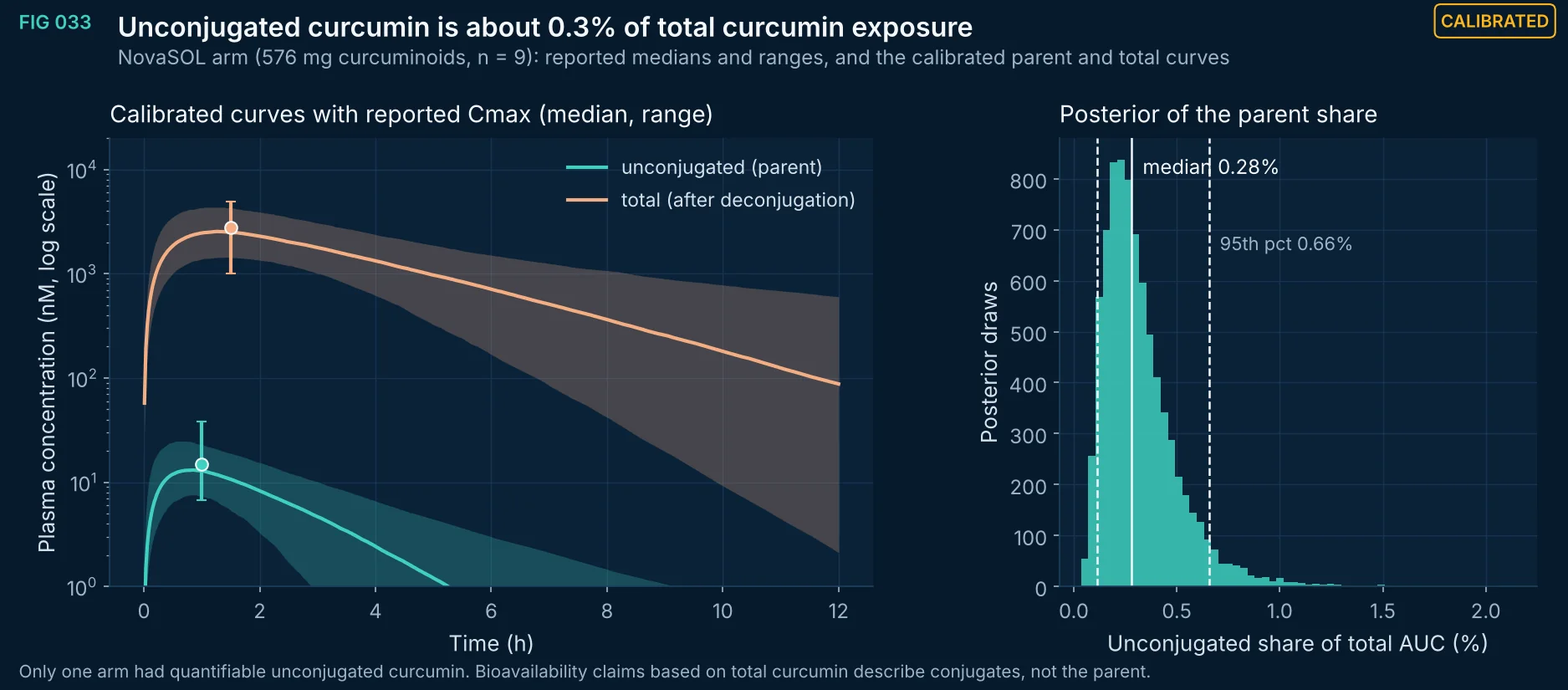
FIG 033Calibrated
Calibrated unconjugated and total curcumin curves for the NovaSOL arm, and the posterior distribution of the unconjugated share of total AUC.
Method, sources and limits
- Method
- Two Bateman curves sharing kₐ; log-normal likelihood on medians (σ_log = ln(max/min)/4) and normal likelihood on Tmax (SD 0.35 h assumed).
- Sources and code
- Kroon MAGM, van Laarhoven HWM, Swart EL, van Tellingen O, Kemper EM. A pharmacokinetic study and critical reappraisal of curcumin formulations enhancing bioavailability. Kroon MAGM et al. A pharmacokinetic study and critical reappraisal of curcumin formulations enhancing bioavailability. Kroon MAGM et al. A pharmacokinetic study and critical reappraisal of curcumin formulations enhancing bioavailability. iScience 2025;28(6):112575, Table 2. doi:10.1016/j.isci.2025.112575
- Supports
- Total and parent curcumin exposures differ by more than two orders of magnitude in this arm.
- Does not support
- Exposure of any other formulation or dose.
- Limitations
- Medians and ranges of n = 9; σ from the range is an approximation.
- The quercetin and berberine metabolite profiles are not modeled: no matched parent and metabolite summary data were extracted.
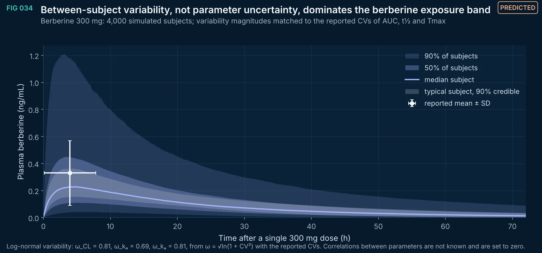
FIG 034Predicted
Simulated concentration–time percentiles for 4,000 subjects after 300 mg berberine, compared with the typical-subject credible band and the reported summary point.
Method, sources and limits
- Method
- Monte Carlo: posterior draws of the typical-subject parameters combined with log-normal between-subject variability (moment-matched to reported CVs).
- Sources and code
- Data: Li G, Zhao M, Qiu F, Sun Y, Zhao L. Pharmacokinetic interactions and tolerability of berberine chloride with simvastatin and fenofibrate: an open-label, randomized, parallel study in healthy Chinese subjects. Drug Des Devel Ther 2019;13:129–139. doi:10.2147/DDDT.S185487 (berberine 300 mg single dose, n = 12, Table 6).
- Supports
- The width of plausible individual exposure after 300 mg.
- Does not support
- Exposure at other doses, in patients or with food.
- Limitations
- Variability magnitudes are moment-matched, not estimated from individual data; parameter correlations assumed zero.
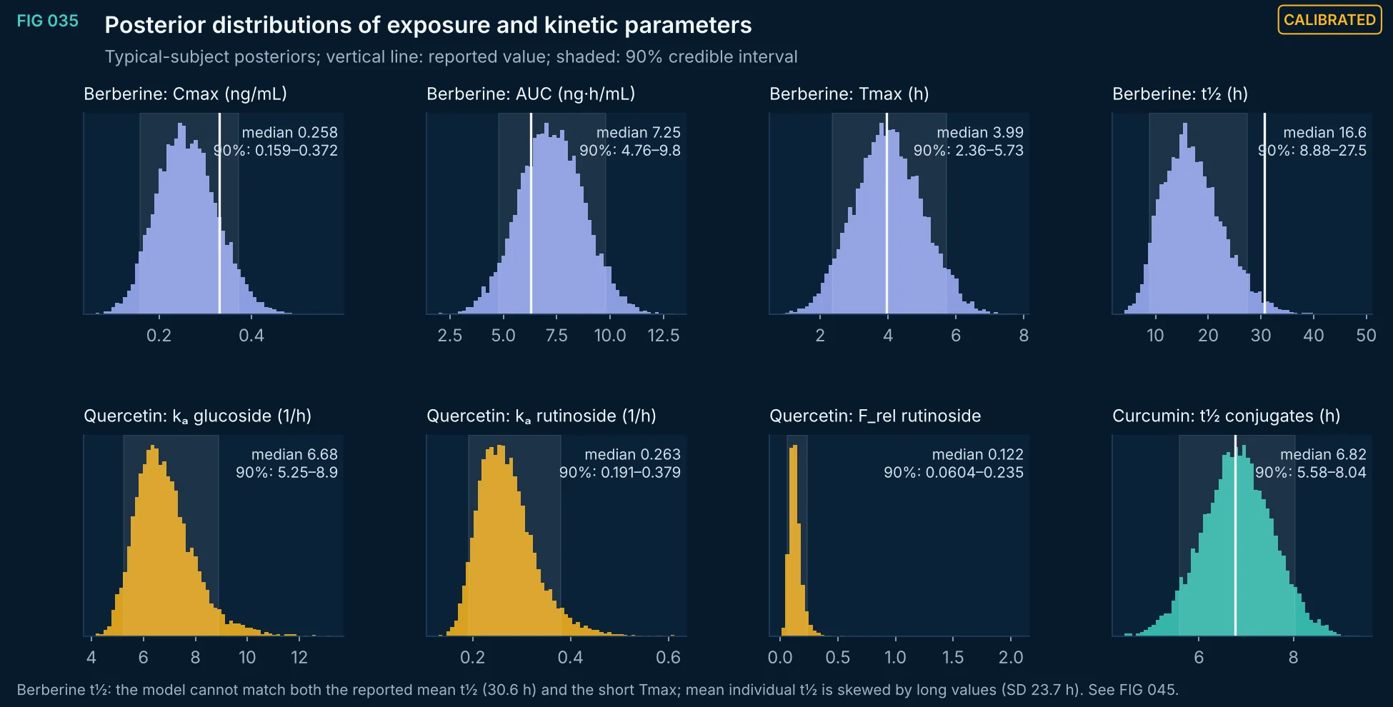
FIG 035Calibrated
Fill each empty list (for example FIG 035 Supports: 'Parameter uncertainty given summary-level data'; Does not support: 'Between-subject variability or individual exposure'), or hide headings whose list is empty.
Method, sources and limits
- Method
- NUTS posterior draws (8,000 per model).
- Sources and code
- Data: Li G, Zhao M, Qiu F, Sun Y, Zhao L. Pharmacokinetic interactions and tolerability of berberine chloride with simvastatin and fenofibrate: an open-label, randomized, parallel study in healthy Chinese subjects. Drug Des Devel Ther 2019;13:129–139. doi:10.2147/DDDT.S185487 (berberine 300 mg single dose, n = 12, Table 6).; Data: Graefe et al., J Clin Pharmacol 2001;41:492–499 (n = 12 crossover).; Data: Vareed et al., Cancer Epidemiol Biomarkers Prev 2008;17:1411–1417; iScience 2025;28:112575.
- Supports
- Does not support
- Limitations
- Summary-level likelihood.
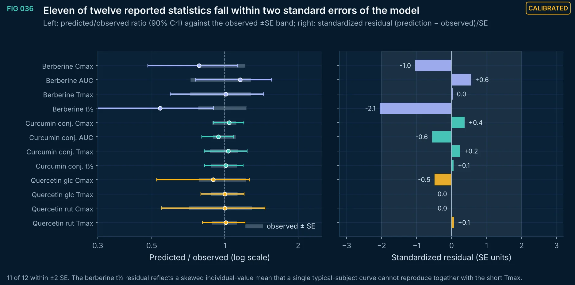
FIG 036Calibrated
Agreement between reported summary statistics and model predictions, with standardized residuals.
Method, sources and limits
- Method
- Posterior medians and 90% intervals vs reported values ± SE.
- Sources and code
- Data: Li G, Zhao M, Qiu F, Sun Y, Zhao L. Pharmacokinetic interactions and tolerability of berberine chloride with simvastatin and fenofibrate: an open-label, randomized, parallel study in healthy Chinese subjects. Drug Des Devel Ther 2019;13:129–139. doi:10.2147/DDDT.S185487 (berberine 300 mg single dose, n = 12, Table 6).; Data: Graefe et al., J Clin Pharmacol 2001;41:492–499 (n = 12 crossover).; Data: Vareed et al., Cancer Epidemiol Biomarkers Prev 2008;17:1411–1417; iScience 2025;28:112575.
- Supports
- Does not support
- Limitations
- These are the calibration data, not independent validation data.
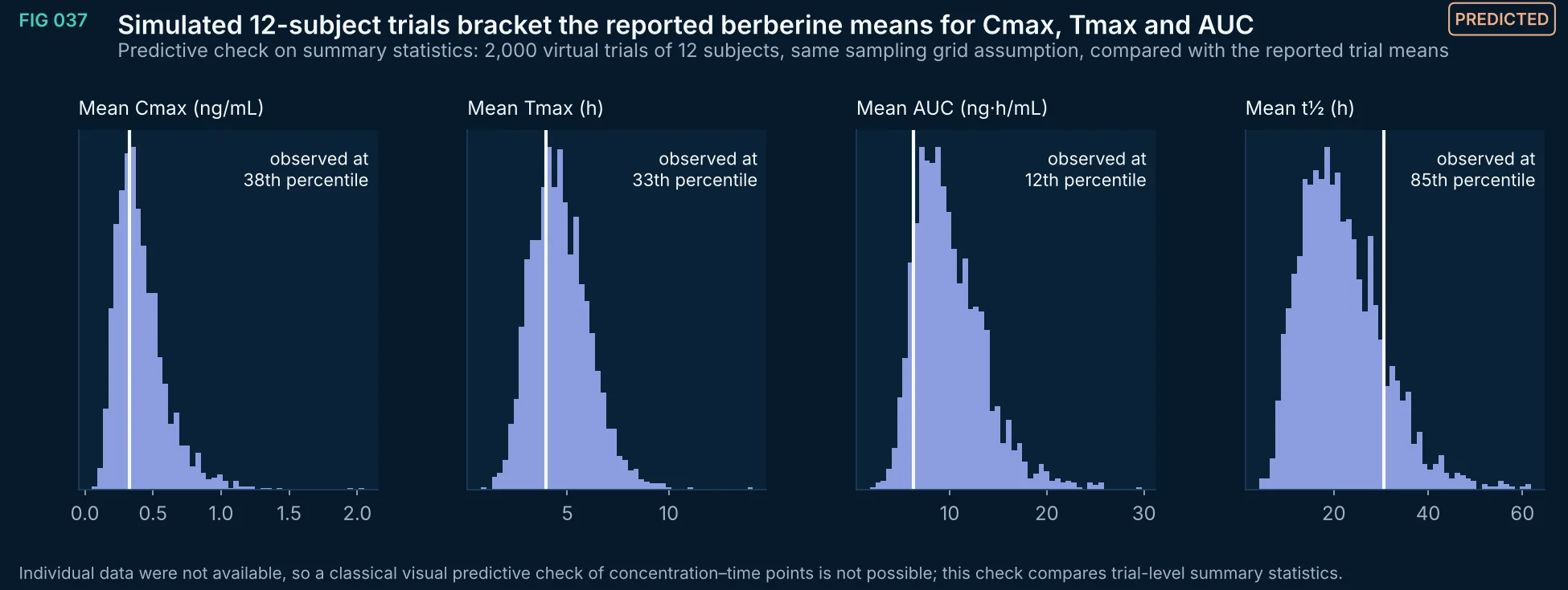
FIG 037Predicted
Fill the empty Supports / Does not support lists for FIG 037, FIG 039 and FIG 045 (e.g., FIG 037 Supports: 'That the calibrated model reproduces 12-subject trial means'; Does not support: 'Validation against independent concentration–time data'), or hide the headings when the list is empty.
Method, sources and limits
- Method
- Posterior draw per trial plus log-normal between-subject variability; sampling grid 0.25–72 h assumed.
- Sources and code
- Data: Li G, Zhao M, Qiu F, Sun Y, Zhao L. Pharmacokinetic interactions and tolerability of berberine chloride with simvastatin and fenofibrate: an open-label, randomized, parallel study in healthy Chinese subjects. Drug Des Devel Ther 2019;13:129–139. doi:10.2147/DDDT.S185487 (berberine 300 mg single dose, n = 12, Table 6).
- Supports
- Does not support
- Limitations
- Not a VPC on observed concentration–time data.
- The sampling schedule of the study is assumed.
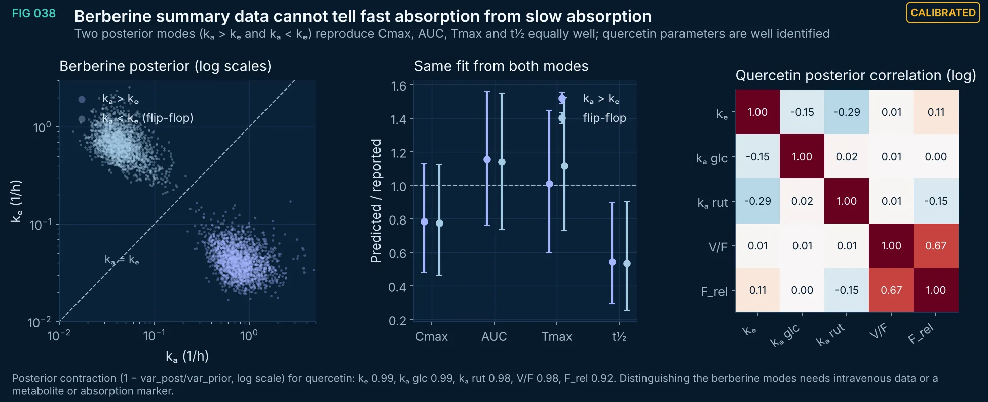
FIG 038Calibrated
Flip-flop non-identifiability of berberine absorption and elimination, and the posterior correlation structure of the quercetin model.
Method, sources and limits
- Method
- Two constrained fits (kₐ > kₑ, kₐ < kₑ); Pearson correlation of log posterior draws; contraction relative to the prior.
- Sources and code
- Data: Li G, Zhao M, Qiu F, Sun Y, Zhao L. Pharmacokinetic interactions and tolerability of berberine chloride with simvastatin and fenofibrate: an open-label, randomized, parallel study in healthy Chinese subjects. Drug Des Devel Ther 2019;13:129–139. doi:10.2147/DDDT.S185487 (berberine 300 mg single dose, n = 12, Table 6).; Data: Graefe et al., J Clin Pharmacol 2001;41:492–499 (n = 12 crossover).
- Supports
- Oral summary data alone cannot establish the rate-limiting step of berberine disposition.
- Does not support
- Any mechanism of berberine absorption or elimination.
- Limitations
- Prior-dependent contraction values.
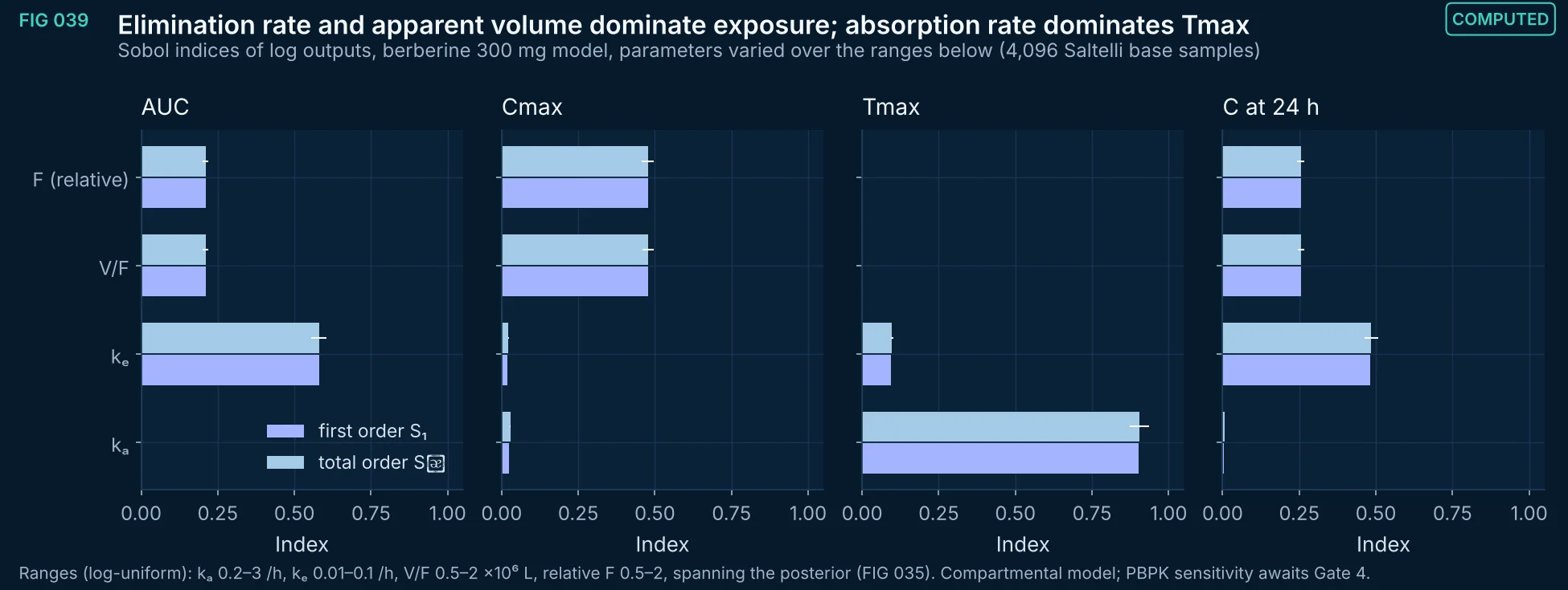
FIG 039Computed
First- and total-order Sobol indices for AUC, Cmax, Tmax and the 24 h concentration of the berberine model.
Method, sources and limits
- Method
- SALib Saltelli sampling and Sobol analysis on log-transformed outputs; 95% bootstrap intervals for Sᴛ.
- Sources and code
- Deduplicate the list to one entry per source (Bernabé-Pineda 2004; Berga 2023; Krasnov BigSolDB 2.0 and its row sources; Hansen 2007; Chen 2024; Li 2018; Guo 2026; Dechayont 2026; Wang 1997; Li G 2019 DDDT; Graefe 2001; Vareed 2008; Kroon 2025; Ghia 1982; Crank 1975; ICH M9, Q3C(R8), Q8(R2), Q9(R1); Rothwell 2005) and remove 'Model calibrated in FIG 032–035.' and 'PK fits, this study.'
- Supports
- Does not support
- Limitations
- Compartmental, not PBPK.
- Indices depend on the chosen ranges.
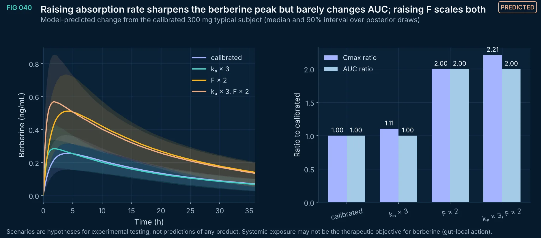
FIG 040Predicted
Predicted concentration–time curves and Cmax/AUC ratios when the absorption rate or the relative bioavailability of berberine is changed.
Method, sources and limits
- Method
- Calibrated posterior with kₐ or F multiplied; all else unchanged.
- Sources and code
- Data: Li G, Zhao M, Qiu F, Sun Y, Zhao L. Pharmacokinetic interactions and tolerability of berberine chloride with simvastatin and fenofibrate: an open-label, randomized, parallel study in healthy Chinese subjects. Drug Des Devel Ther 2019;13:129–139. doi:10.2147/DDDT.S185487 (berberine 300 mg single dose, n = 12, Table 6).
- Supports
- Which kinetic lever a formulation would have to move to change Cmax vs AUC.
- Does not support
- That any formulation achieves these changes.
- Limitations
- Assumes linear kinetics and unchanged elimination.
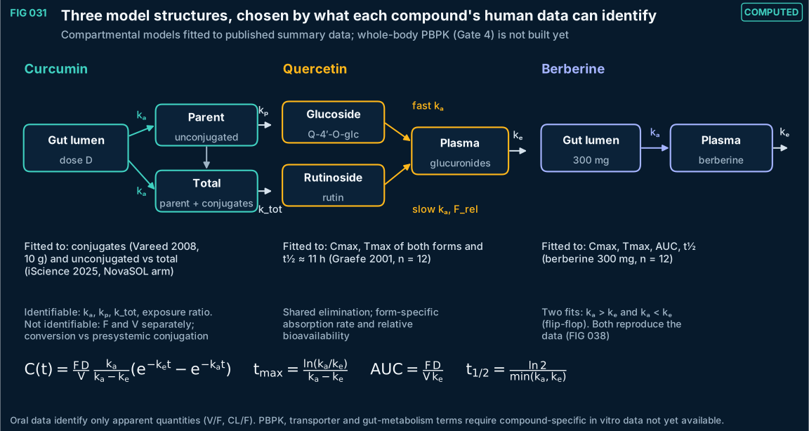
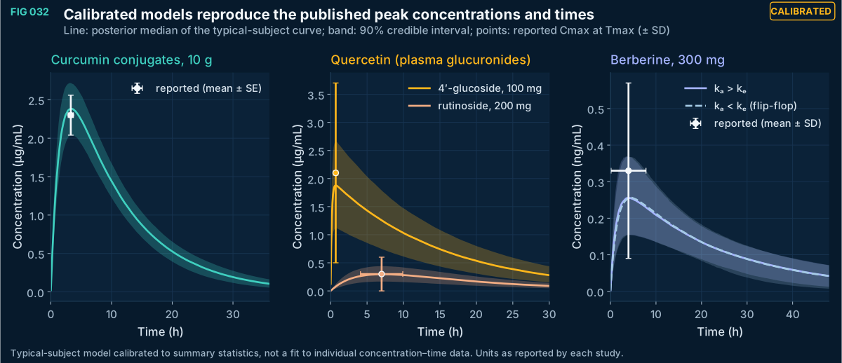
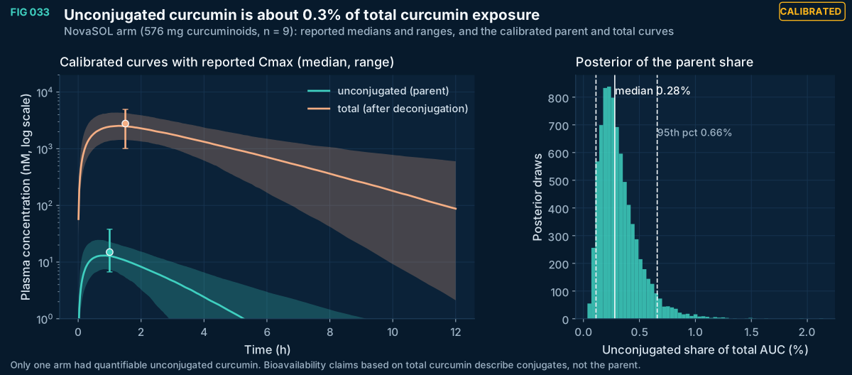
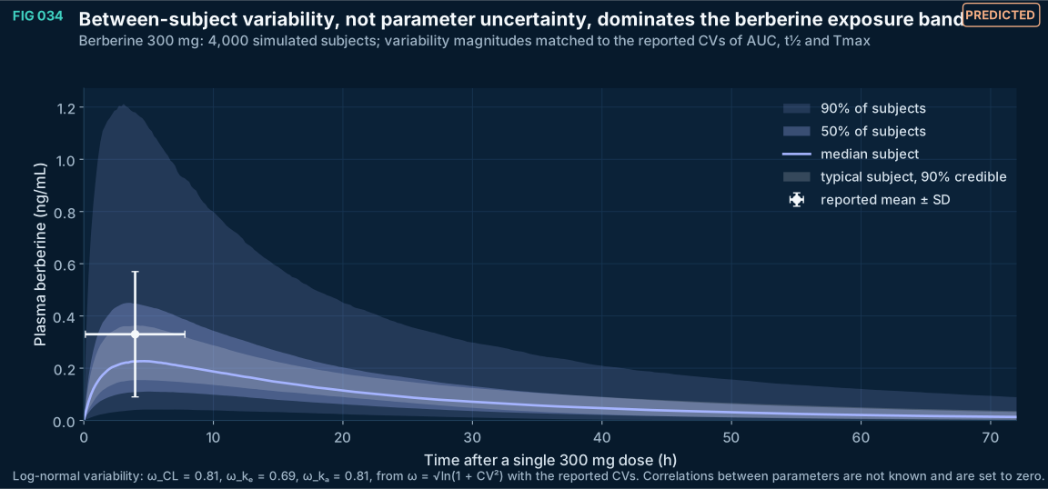
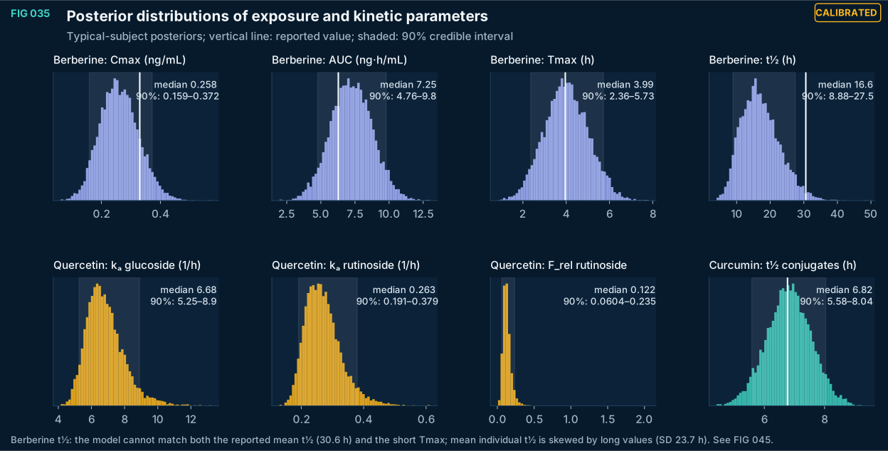
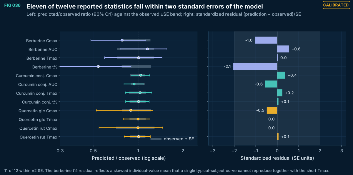
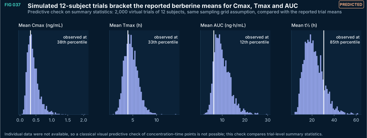
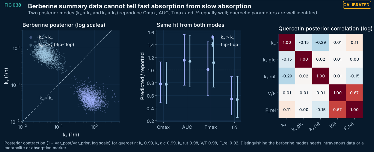
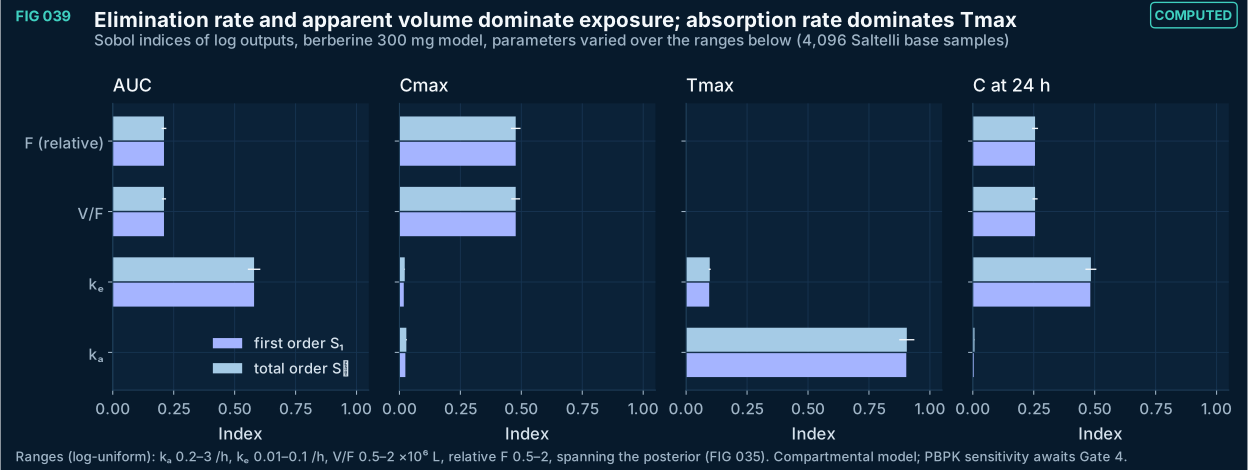
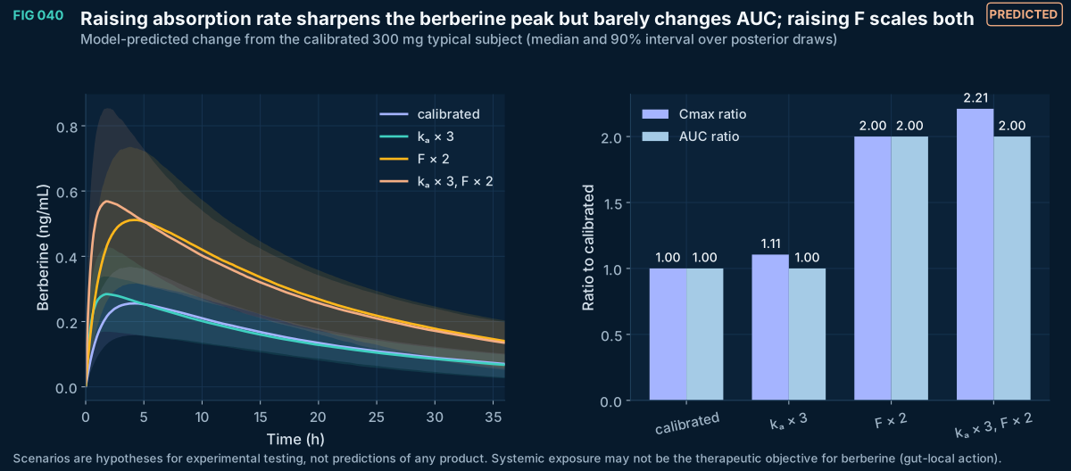
FIG 041–053
Uncertainty and inference
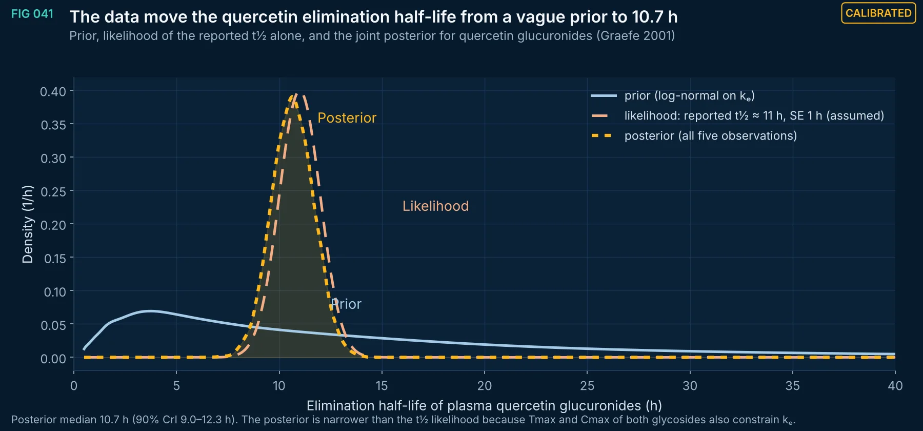
FIG 041Calibrated
Fill the empty lists (e.g., FIG 041 Supports: 'How much the single reported t½ constrains the model'; Does not support: 'A half-life for free quercetin') or hide headings with no items.
Method, sources and limits
- Method
- Kernel density of prior predictive and posterior draws; the likelihood curve is the normalized normal likelihood of the t½ observation alone.
- Sources and code
- Data: Graefe et al., J Clin Pharmacol 2001;41:492–499 (n = 12 crossover).
- Supports
- Does not support
- Limitations
- The SE of the 'about 11 h' t½ is an assumption (1 h).
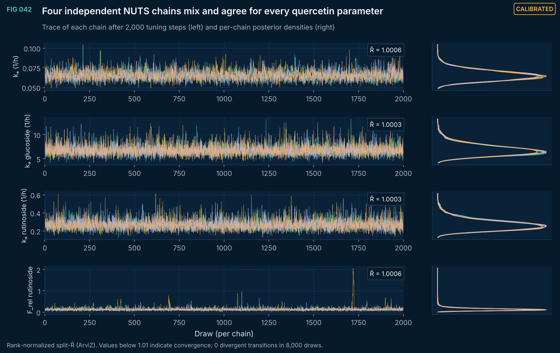
FIG 042Calibrated
Per-chain traces and densities of the quercetin model parameters.
Method, sources and limits
- Method
- PyMC NUTS, target acceptance 0.97, 4 chains.
- Sources and code
- Data: Graefe et al., J Clin Pharmacol 2001;41:492–499 (n = 12 crossover).
- Supports
- Does not support
- Limitations
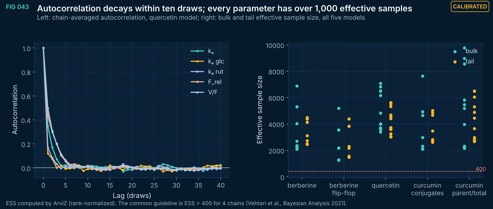
FIG 043Calibrated
Chain autocorrelation for the quercetin model and bulk/tail ESS for every parameter of every PK model.
Method, sources and limits
- Method
- ArviZ ess (bulk, tail).
- Sources and code
- PK fits, this study.
- Supports
- Does not support
- Limitations
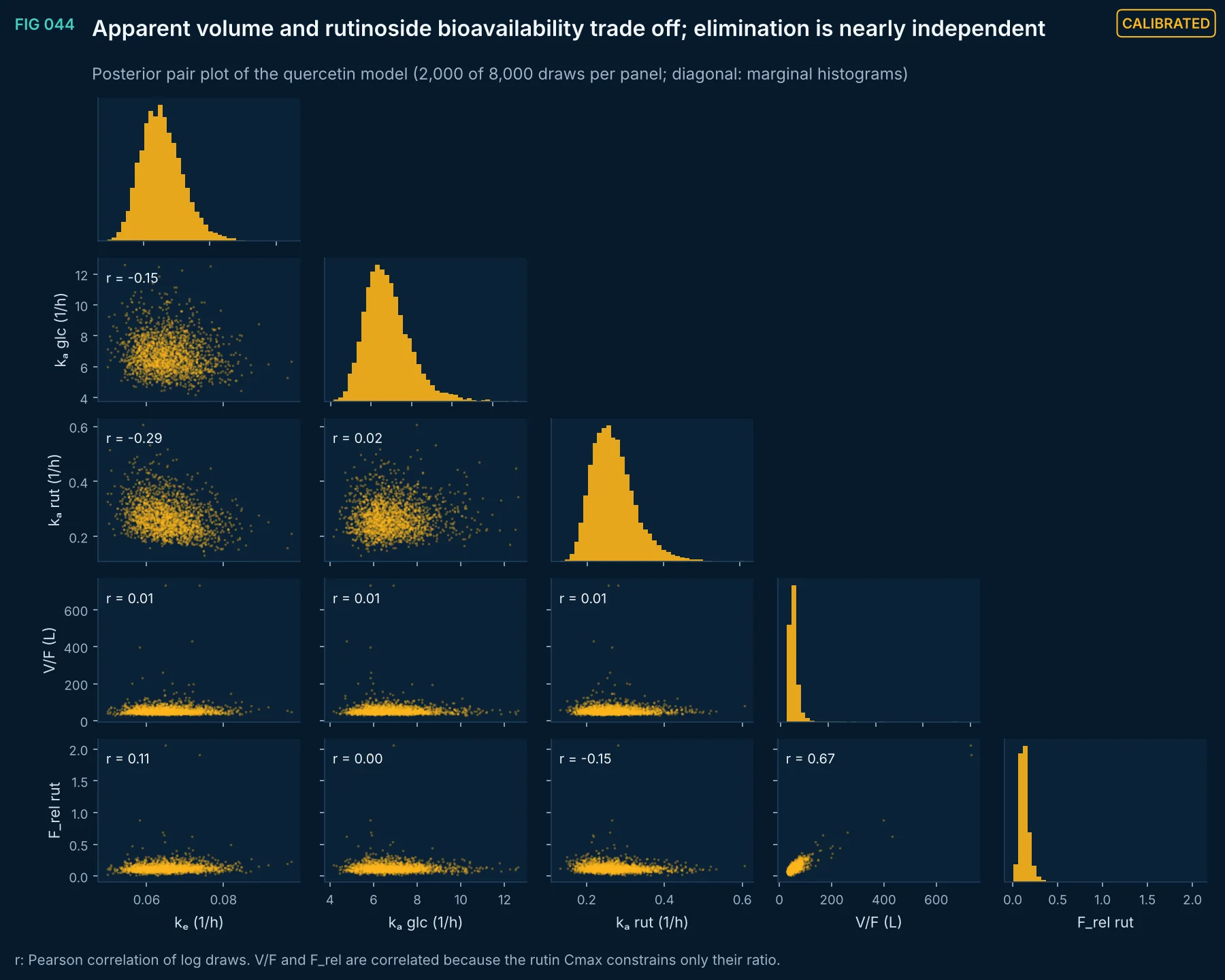
FIG 044Calibrated
Posterior pair plot of the quercetin PK parameters.
Method, sources and limits
- Method
- NUTS draws.
- Sources and code
- Data: Graefe et al., J Clin Pharmacol 2001;41:492–499 (n = 12 crossover).
- Supports
- Does not support
- Limitations
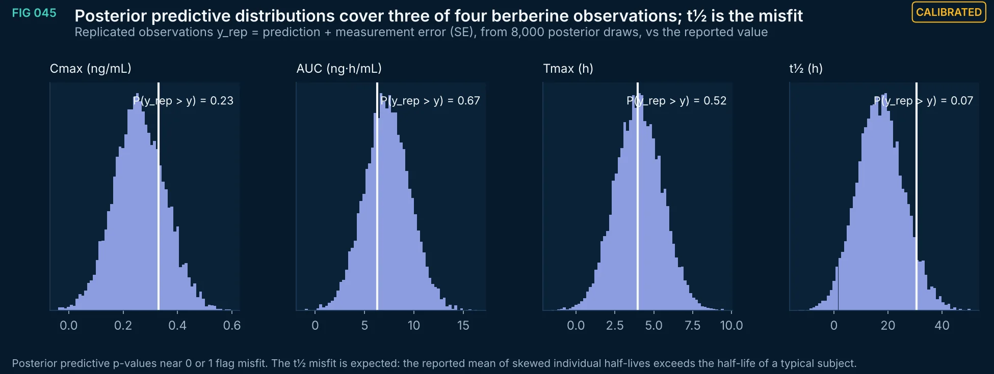
FIG 045Calibrated
Posterior predictive distributions of the four berberine summary statistics with the observed values and posterior predictive p-values.
Method, sources and limits
- Method
- y_rep = posterior prediction + N(0, SE) measurement error.
- Sources and code
- Data: Li G, Zhao M, Qiu F, Sun Y, Zhao L. Pharmacokinetic interactions and tolerability of berberine chloride with simvastatin and fenofibrate: an open-label, randomized, parallel study in healthy Chinese subjects. Drug Des Devel Ther 2019;13:129–139. doi:10.2147/DDDT.S185487 (berberine 300 mg single dose, n = 12, Table 6).
- Supports
- Does not support
- Limitations
- Calibration data, not independent data.
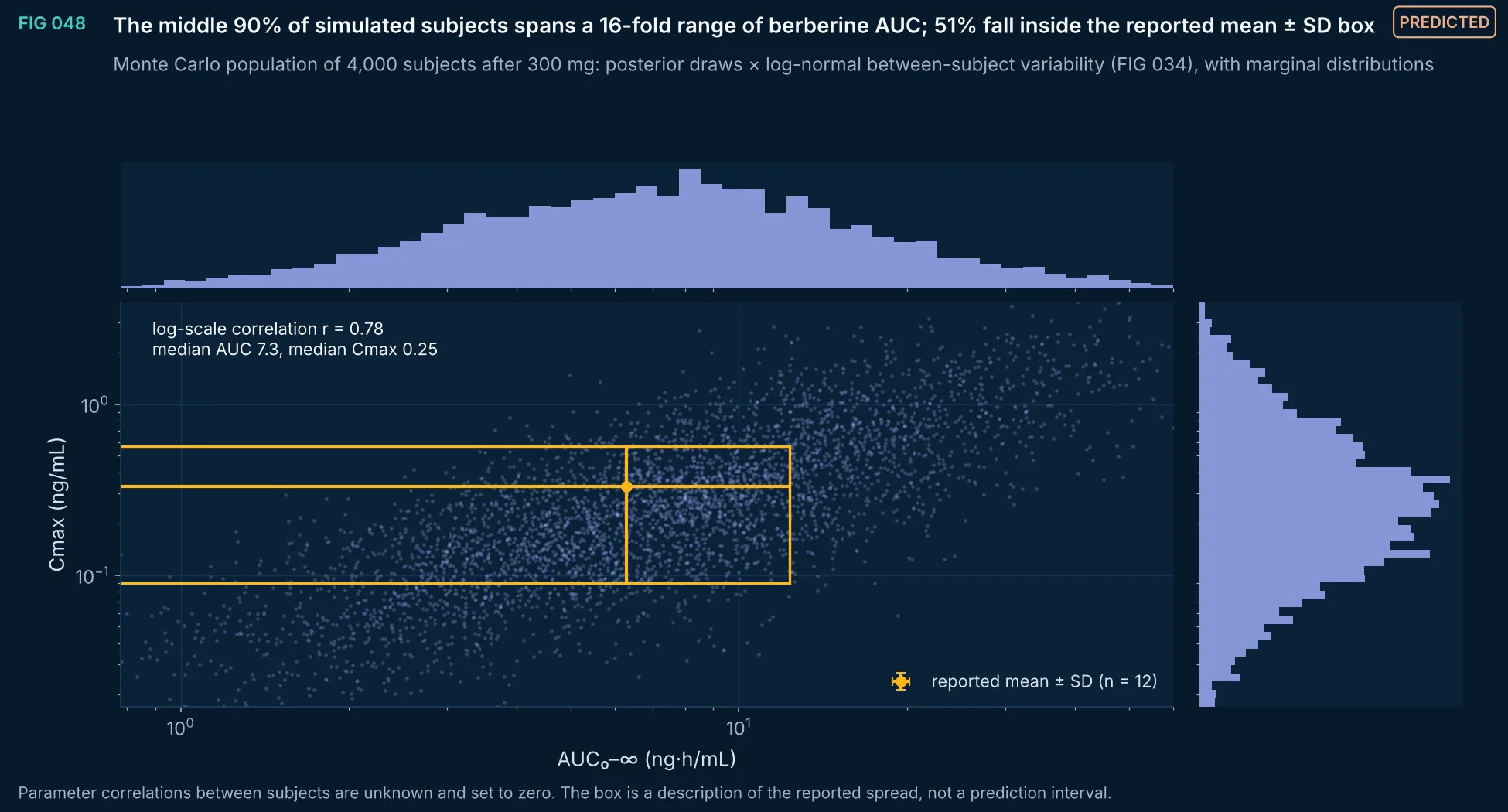
FIG 048Predicted
Joint distribution of AUC and Cmax in a simulated population given berberine 300 mg, combining posterior uncertainty in the typical-subject model with between-subject variability matched to the reported coefficients of variation. Marginal histograms show the skewed, log-normal shape that a mean ± SD summary hides.
Method, sources and limits
- Method
- Posterior draws from the summary-level calibration (FIG 035) × independent log-normal variability on CL/F, kₑ and kₐ; analytic Bateman Cmax and AUC.
- Sources and code
- Li G, Zhao M, Qiu F, Sun Y, Zhao L. Pharmacokinetic interactions and tolerability of berberine chloride with simvastatin and fenofibrate: an open-label, randomized, parallel study in healthy Chinese subjects. Drug Des Devel Ther 2019;13:129–139. doi:10.2147/DDDT.S185487 (berberine 300 mg single dose, n = 12, Table 6). Scripts 06_PK_PBPK/pk_fit.py and 07_MCMC_uncertainty/mc_figs.py.
- Supports
- Expect wide between-subject exposure differences in any berberine study and size studies accordingly.
- Does not support
- Exposure of any formulation other than the studied one.
- Limitations
- Variability magnitudes inferred from summary CVs, not from individual data.
- No covariates (sex, body weight, genotype, food).
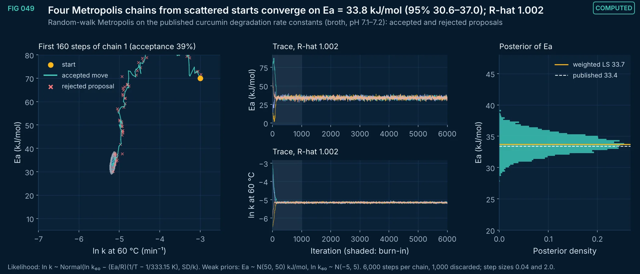
FIG 049Computed
A random-walk Metropolis sampler applied to the published first-order rate constants for curcumin in broth (Dechayont et al. 2026). Left: accepted moves and rejected proposals on the posterior density during the first 160 steps. Middle: four chains started far apart mix within the burn-in window. Right: the posterior of the activation energy agrees with weighted least squares (33.7 kJ/mol) and with the published 33.4 kJ/mol.
Method, sources and limits
- Method
- Random-walk Metropolis, Gaussian proposals, 4 chains × 6,000 iterations, burn-in 1,000; Gelman–Rubin R-hat on post-burn-in draws; temperature-centered parameterization at 60 °C.
- Sources and code
- Dechayont B, Brunaugh AD. Chitosan stabilizes curcumin against hydrolysis and potentiates antimicrobial activity against Pseudomonas aeruginosa in a pH-dependent manner. ACS Omega 2026;11(31):46088–46104. doi:10.1021/acsomega.6c02415. PMID 42597930, PMC13470882 Script 07_MCMC_uncertainty/mc_figs.py.
- Supports
- How a posterior for kinetic parameters is obtained and checked.
- Does not support
- Kinetics outside the measured medium and temperature range.
- Limitations
- Same data and caveats as FIG 025.
- Metropolis is shown for transparency; the PK calibrations (FIG 035–045) use NUTS.
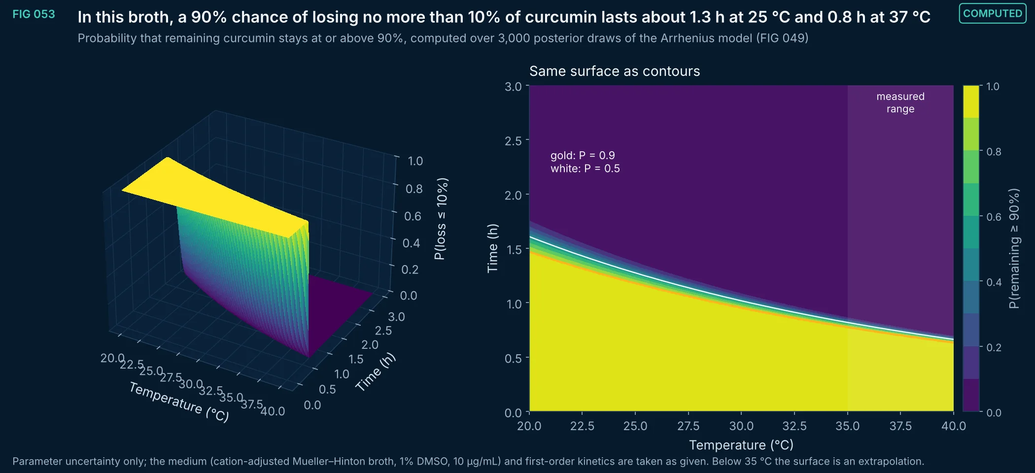
FIG 053Computed
Posterior probability that at least 90% of curcumin remains, as a function of temperature and time, from the Arrhenius posterior fitted to published broth data. The 90% contour is the kind of boundary a stability specification would be set against; for this matrix it is measured in hours, which is why formulation or matrix change is needed before any room-temperature claim.
Method, sources and limits
- Method
- Monte Carlo over 3,000 posterior draws (FIG 049); first-order loss exp(−k(T)t) evaluated on a 41 × 41 grid.
- Sources and code
- Dechayont B, Brunaugh AD. Chitosan stabilizes curcumin against hydrolysis and potentiates antimicrobial activity against Pseudomonas aeruginosa in a pH-dependent manner. ACS Omega 2026;11(31):46088–46104. doi:10.1021/acsomega.6c02415. PMID 42597930, PMC13470882 Script 07_MCMC_uncertainty/mc_figs.py.
- Supports
- How a probability-of-compliance boundary is computed from kinetic data.
- Does not support
- A shelf life for any product or matrix.
- Limitations
- Extrapolation below 35 °C assumes one mechanism.
- Batch-to-batch and analytical variability are not included; the probability reflects parameter uncertainty only.
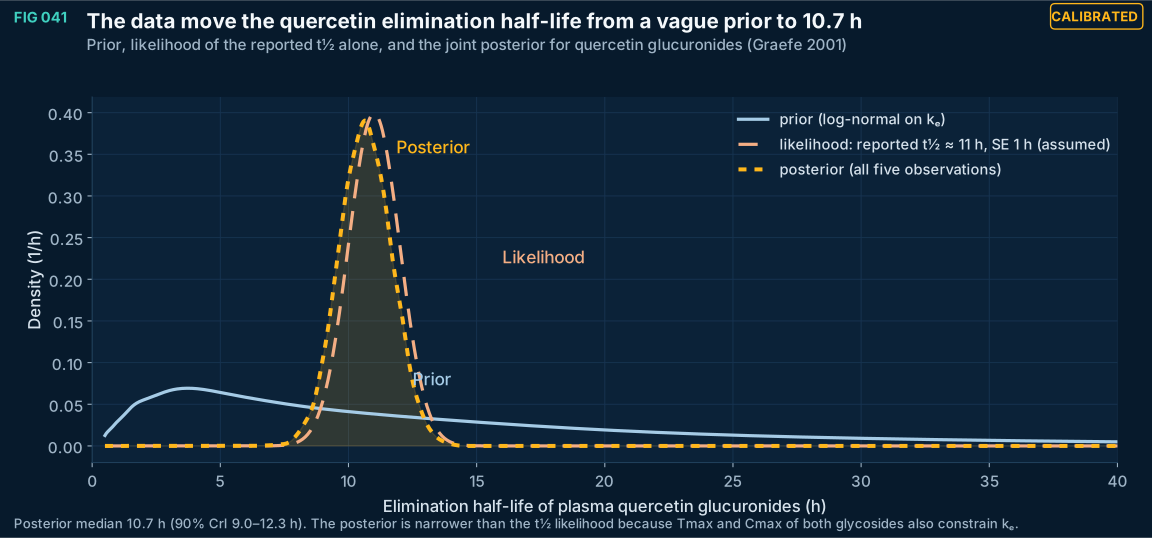
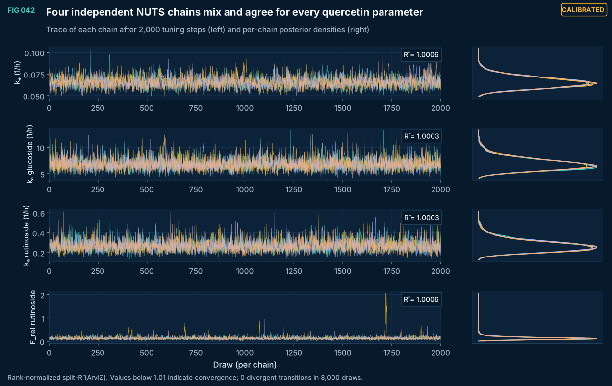
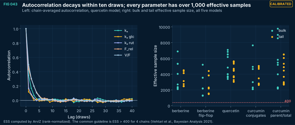
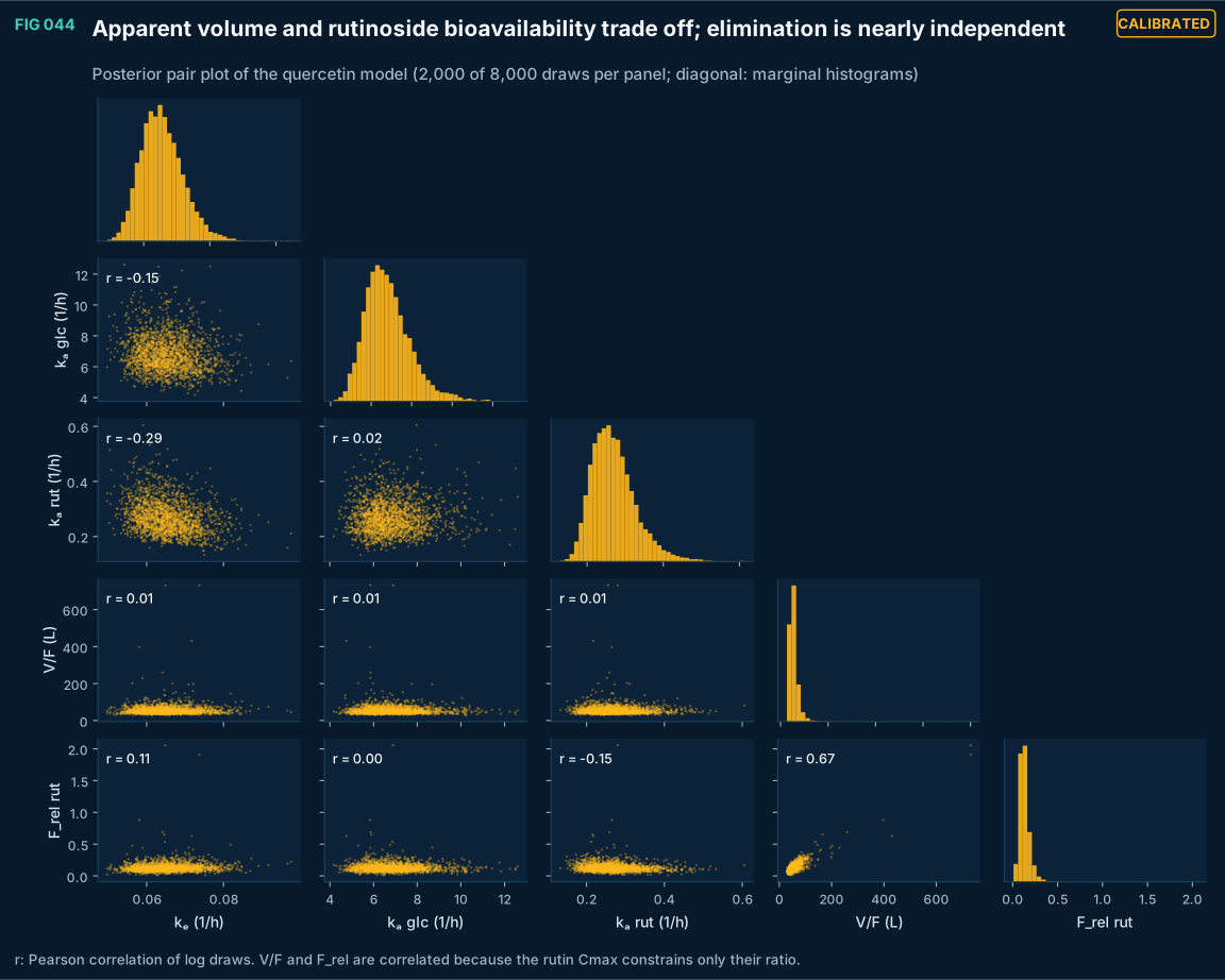
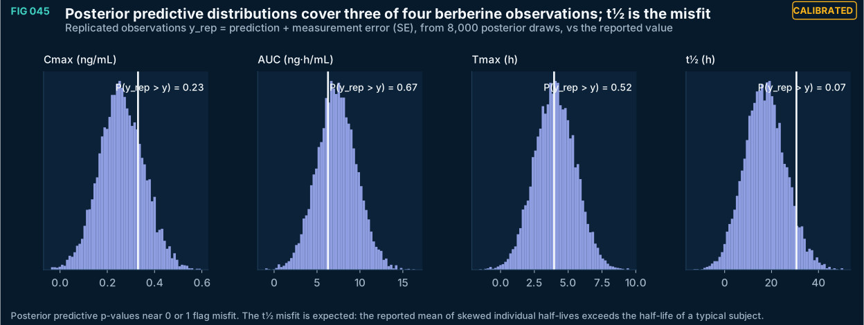
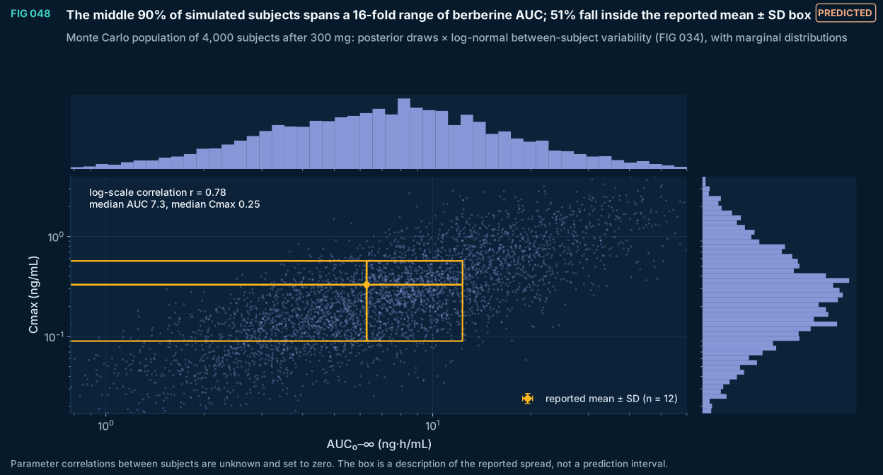
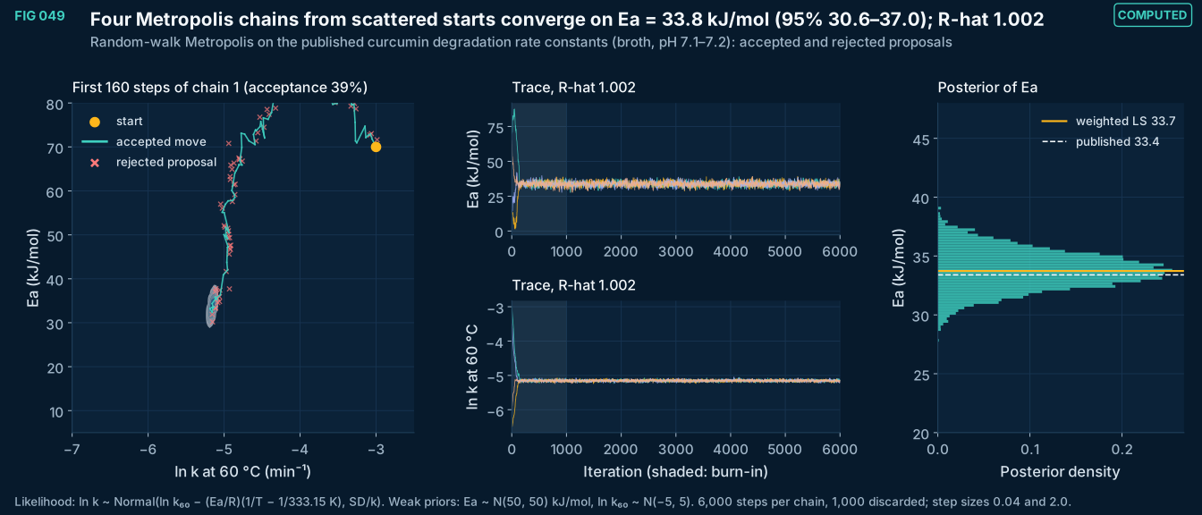
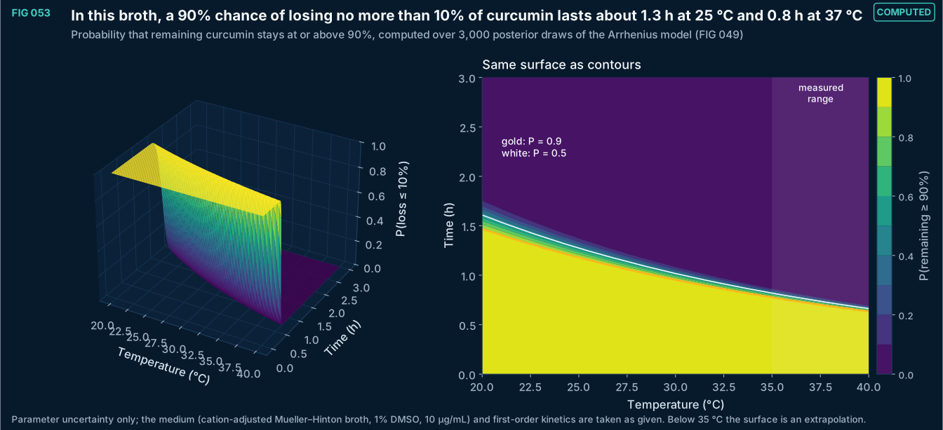
FIG 046–060
Optimization and design space
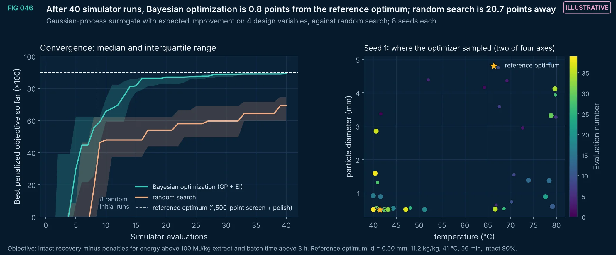
FIG 046Illustrative
Bayesian optimization (Gaussian process with Matérn 5/2 kernel and expected improvement) against random search on the illustrative extraction simulator, with a penalized objective for energy and batch time. With the same 40-evaluation budget, the surrogate-guided search gets closer to the reference optimum and with less spread across seeds. With a real plant or laboratory, each evaluation is an experiment, which is the reason to use such a method.
Method, sources and limits
- Method
- scikit-learn GaussianProcessRegressor (Matérn ν = 5/2, ARD, white noise), EI with ξ = 0.005 maximized over 5,000 random and local candidates; 8 initial random points; 8 independent seeds.
- Sources and code
- Illustrative extraction simulator of FIG 016 (Crank eq. 6.30 with Arrhenius diffusion and degradation; Python port of the EUTECNIQ process-engineering page model). Script 08_multiobjective_optimization/opt_figs.py.
- Supports
- Sequential experimental design as a way to reduce the number of development runs.
- Does not support
- Any optimal process setting for a real extraction.
- Limitations
- The objective is an illustrative simulator, not a plant; the optimization method, not the optimum, is the result.
- All material parameters are assumptions (FIG 016–018).
- Noise-free simulator; real experiments add measurement noise and batch effects.
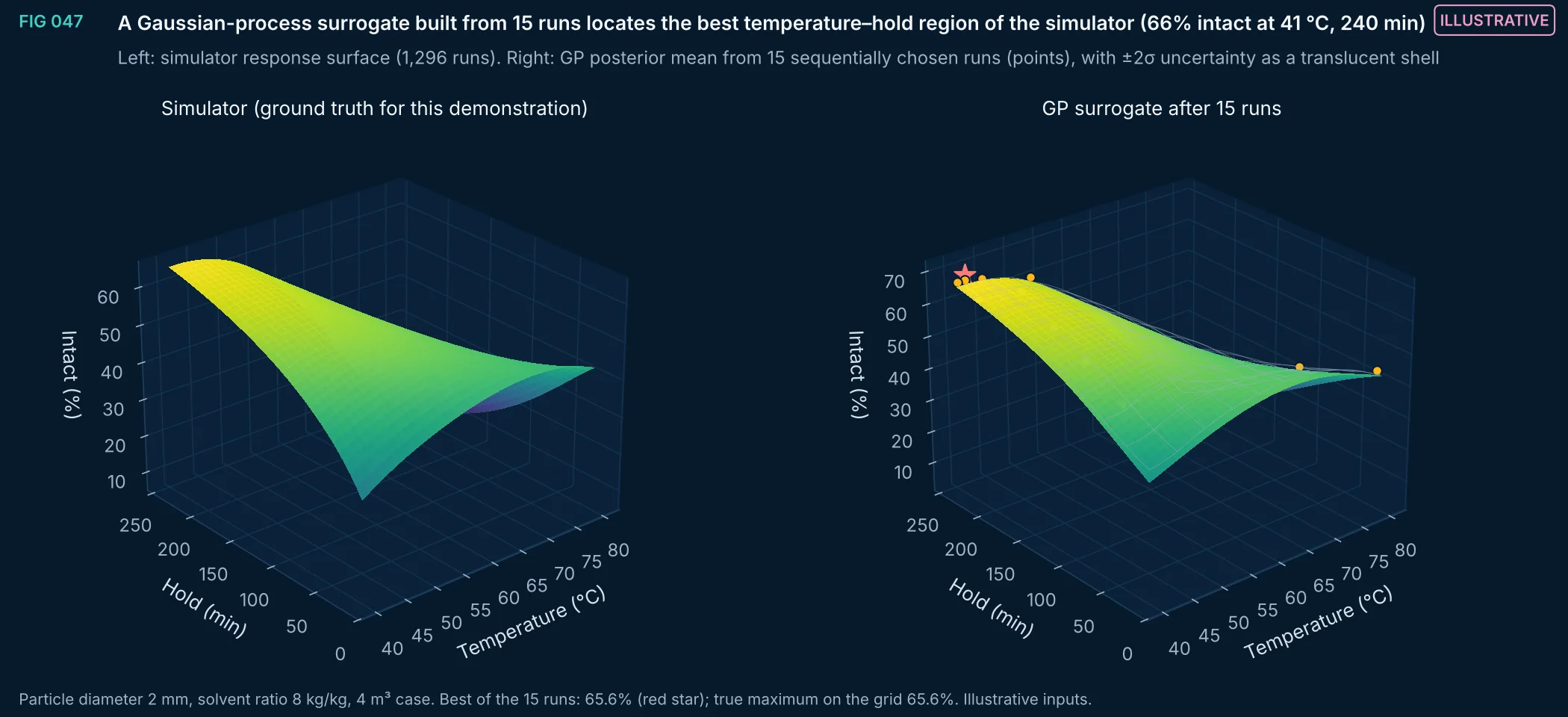
FIG 047Illustrative
Response surface of intact recovery against temperature and hold time from the illustrative simulator, and the Gaussian-process posterior mean built from 15 runs chosen by expected improvement. The surrogate reproduces the ridge of good conditions with far fewer evaluations than the full grid, and its uncertainty shell shows where more runs would be informative.
Method, sources and limits
- Method
- As FIG 046, two inputs; 5 random initial runs, 10 EI-selected runs; GP posterior mean and standard deviation on a 36 × 36 grid.
- Sources and code
- Illustrative extraction simulator of FIG 016 (Crank eq. 6.30 with Arrhenius diffusion and degradation; Python port of the EUTECNIQ process-engineering page model). Script 08_multiobjective_optimization/opt_figs.py.
- Supports
- Visualizing what a surrogate learns from few experiments.
- Does not support
- Process settings for real material.
- Limitations
- The objective is an illustrative simulator, not a plant; the optimization method, not the optimum, is the result.
- All material parameters are assumptions (FIG 016–018).
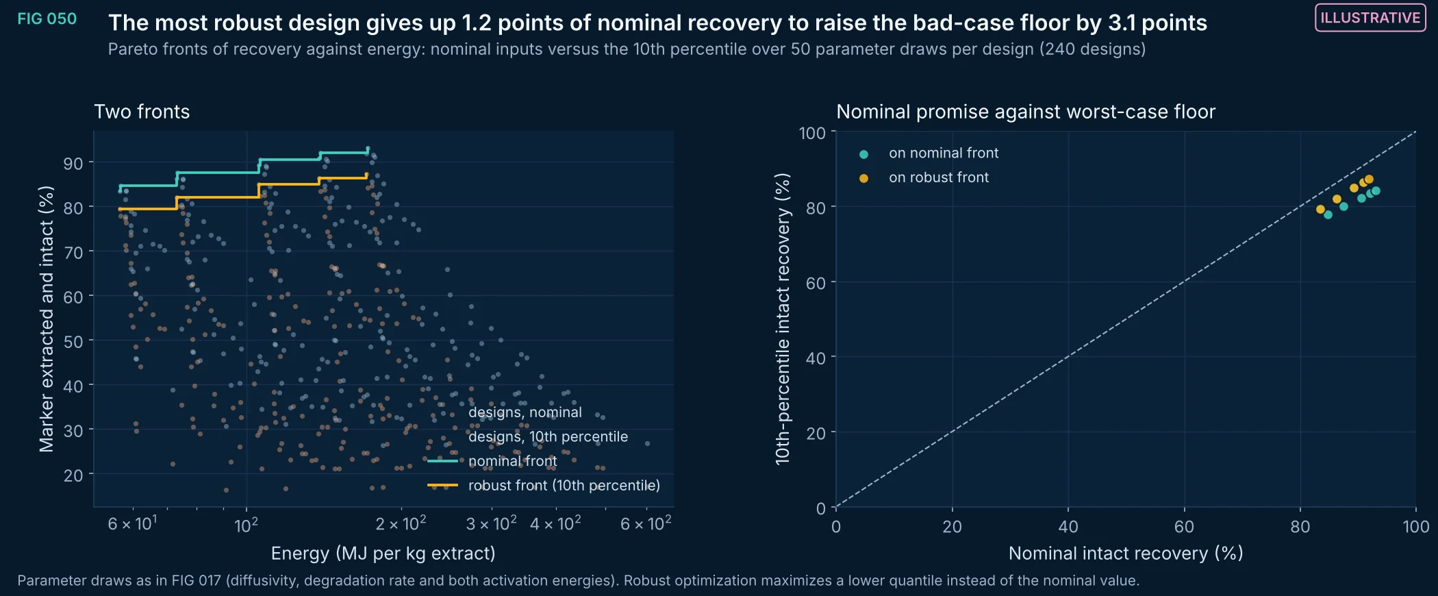
FIG 050Illustrative
For each of 240 extraction designs, intact recovery with nominal inputs and its 10th percentile across 50 draws of the uncertain material parameters, against energy per kilogram of extract. The robust front sits several points below the nominal front, and the design with the best bad-case floor is not the design with the best nominal recovery; optimizing a lower quantile, or measuring the uncertain parameters, changes the choice.
Method, sources and limits
- Method
- Full factorial 4 × 5 × 4 × 3; Monte Carlo with 50 draws per design (seed 11); non-dominated filtering by energy.
- Sources and code
- Illustrative extraction simulator of FIG 016 (Crank eq. 6.30 with Arrhenius diffusion and degradation; Python port of the EUTECNIQ process-engineering page model). Script 08_multiobjective_optimization/opt_figs.py.
- Supports
- Choosing process settings with explicit attention to downside performance.
- Does not support
- A specific robust process for a real material.
- Limitations
- The objective is an illustrative simulator, not a plant; the optimization method, not the optimum, is the result.
- All material parameters are assumptions (FIG 016–018).
- 50 draws per design give quantiles to within a few percentage points.
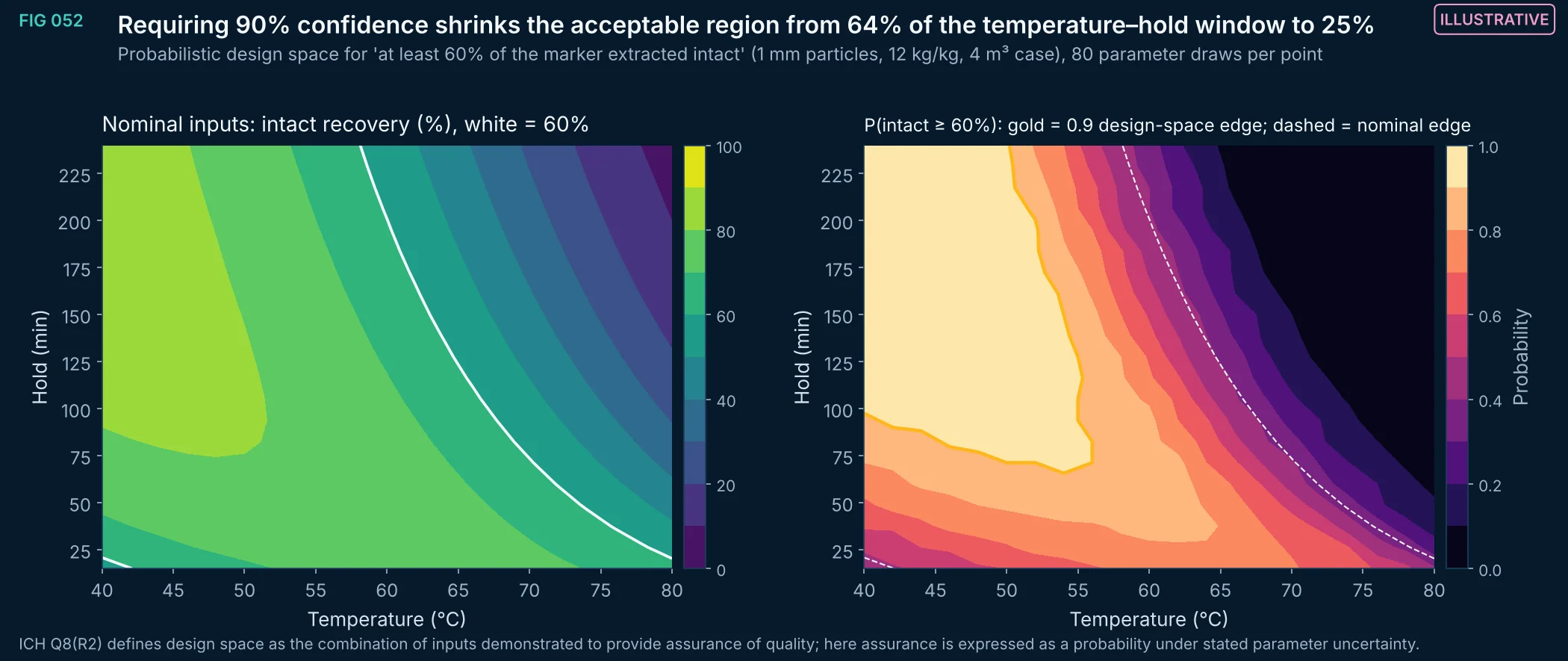
FIG 052Illustrative
Nominal response surface (left) and the probability of meeting the target under parameter uncertainty (right) over temperature and hold time. The region where the target is met with 90% probability is much smaller than the region where the nominal model meets it; a design space defined on nominal predictions would overstate the assurance.
Method, sources and limits
- Method
- Monte Carlo (80 draws per grid point, 21 × 21 grid) of the FIG 016 simulator; probability contour at 0.9.
- Sources and code
- Illustrative extraction simulator of FIG 016 (Crank eq. 6.30 with Arrhenius diffusion and degradation; Python port of the EUTECNIQ process-engineering page model). Script 08_multiobjective_optimization/opt_figs.py. ICH Q8(R2) Pharmaceutical Development (2009), definition of design space.
- Supports
- Expressing a design space as a probability of meeting specifications.
- Does not support
- A design space for any real process.
- Limitations
- The objective is an illustrative simulator, not a plant; the optimization method, not the optimum, is the result.
- All material parameters are assumptions (FIG 016–018).
- Target of 60% intact is an arbitrary illustration.
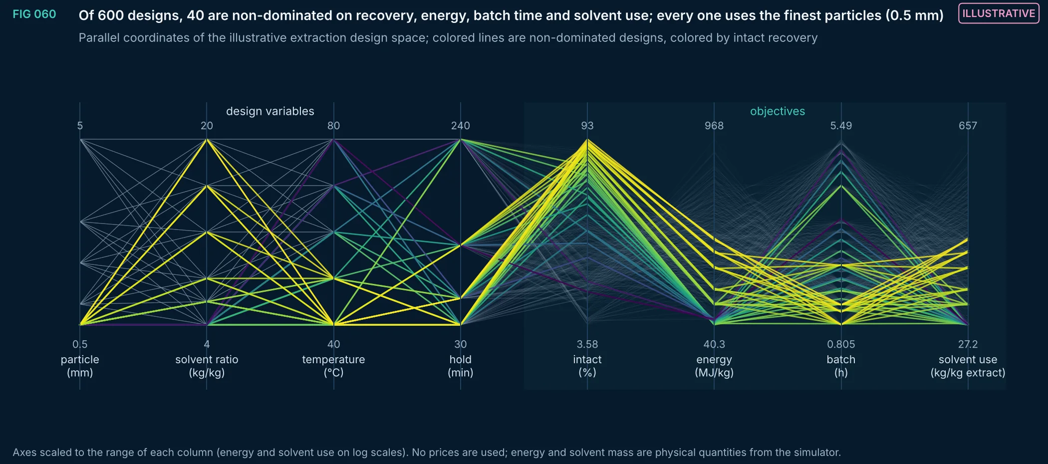
FIG 060Illustrative
Every design of the illustrative full-factorial sweep drawn as a line across its four inputs and four outcomes, with the non-dominated designs highlighted. The view shows at once which input ranges are compatible with good trade-offs, without collapsing the objectives into a single score or a price.
Method, sources and limits
- Method
- 5 × 6 × 5 × 4 factorial of the FIG 016 simulator; four-objective non-dominated filtering (maximize intact; minimize energy, batch time and solvent per kg extract).
- Sources and code
- Illustrative extraction simulator of FIG 016 (Crank eq. 6.30 with Arrhenius diffusion and degradation; Python port of the EUTECNIQ process-engineering page model). Script 08_multiobjective_optimization/opt_figs.py.
- Supports
- Communicating a multi-objective trade-off without economic assumptions.
- Does not support
- A process or cost recommendation.
- Limitations
- The objective is an illustrative simulator, not a plant; the optimization method, not the optimum, is the result.
- All material parameters are assumptions (FIG 016–018).
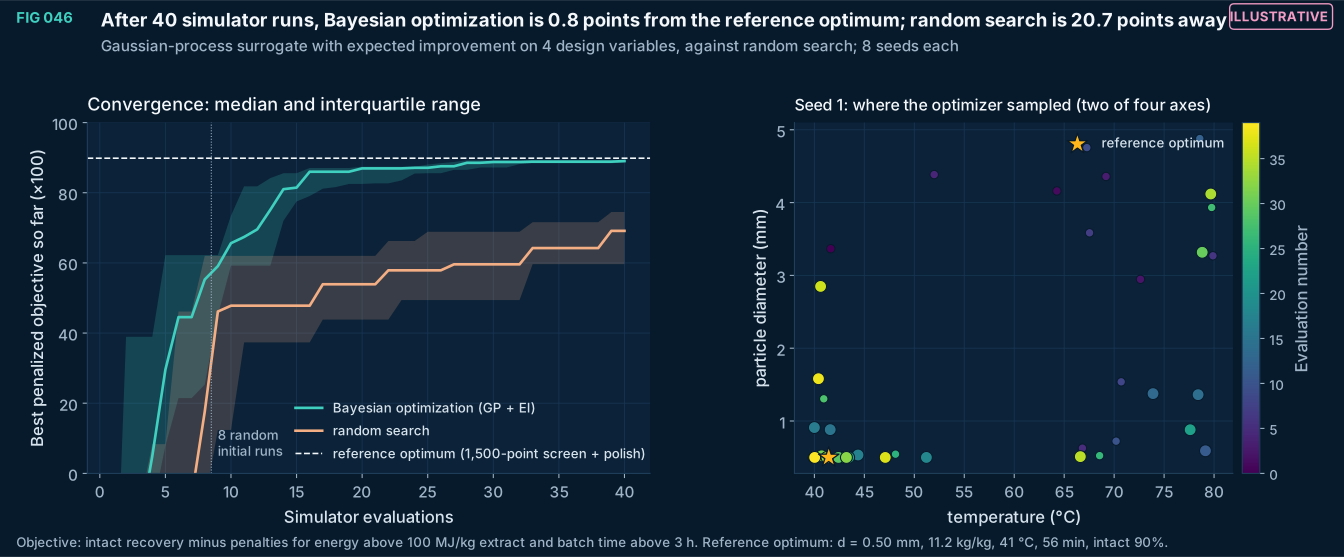
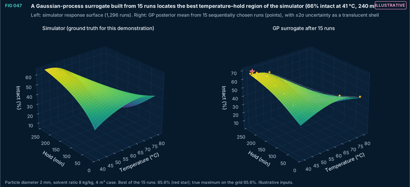
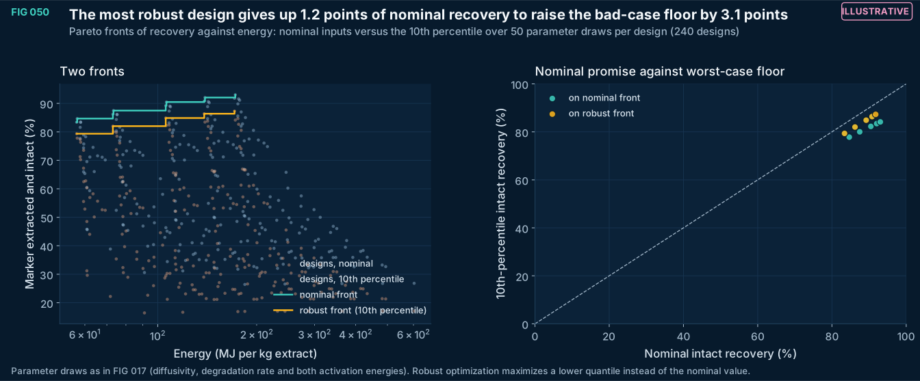
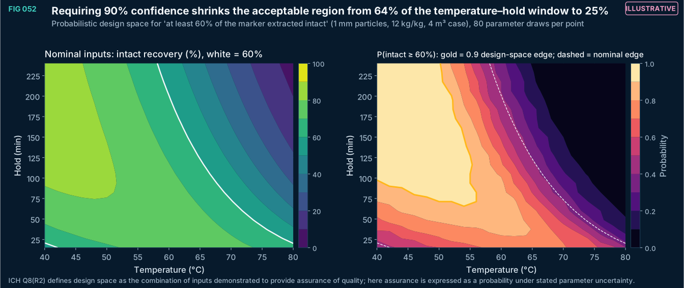
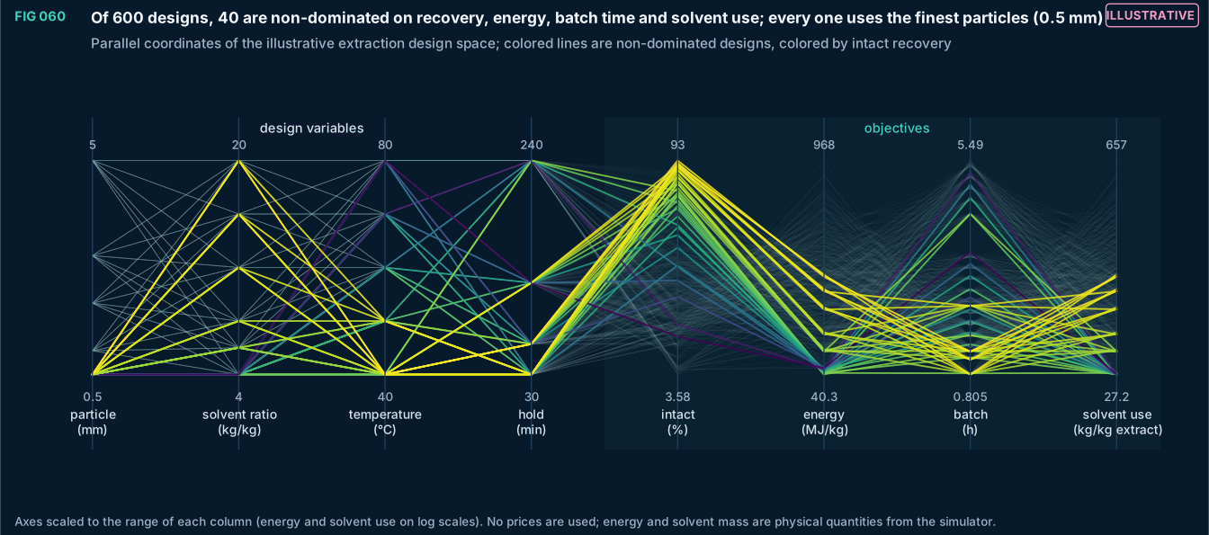
FIG 054–059
Quality systems and validation
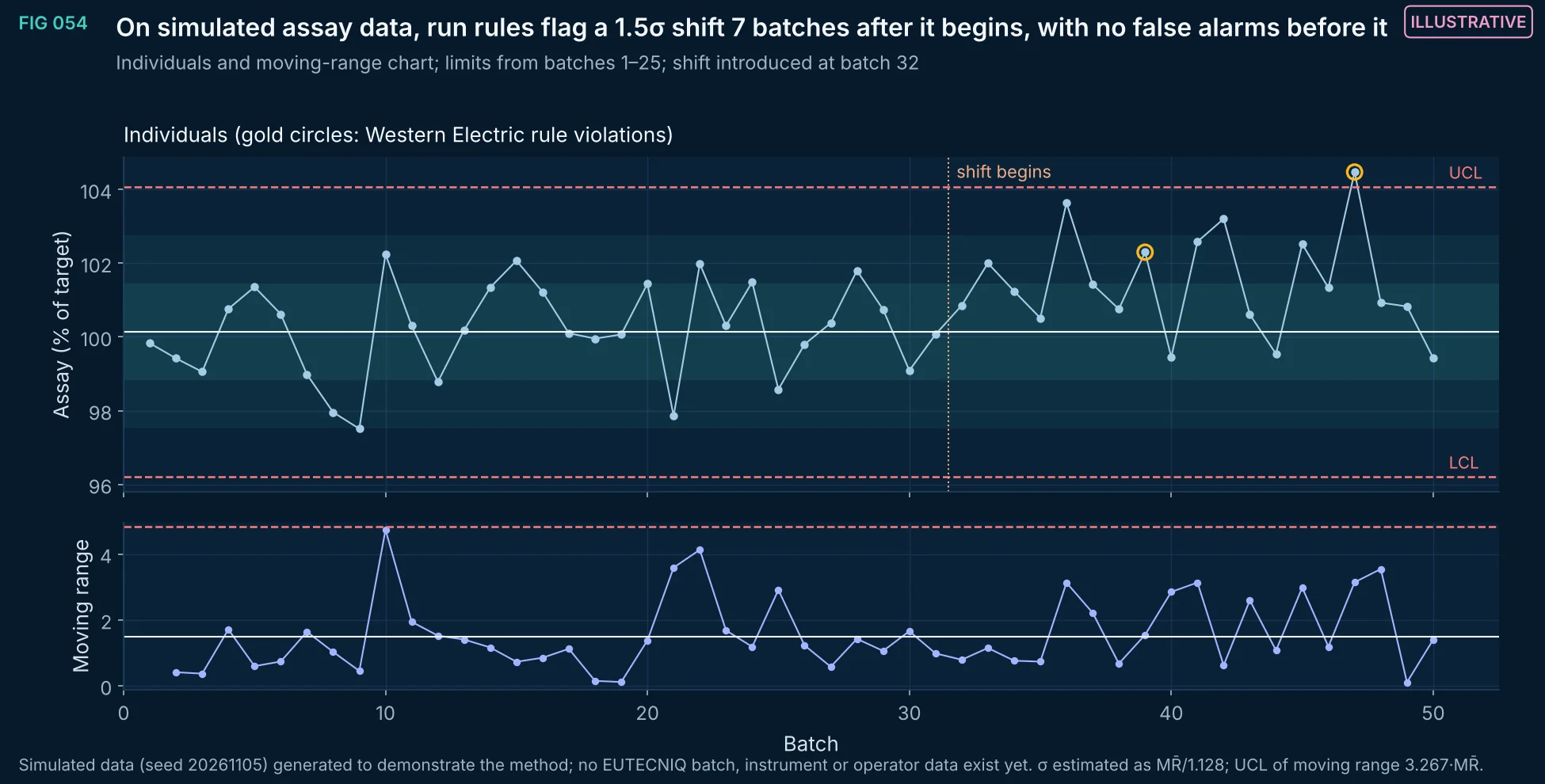
FIG 054Illustrative
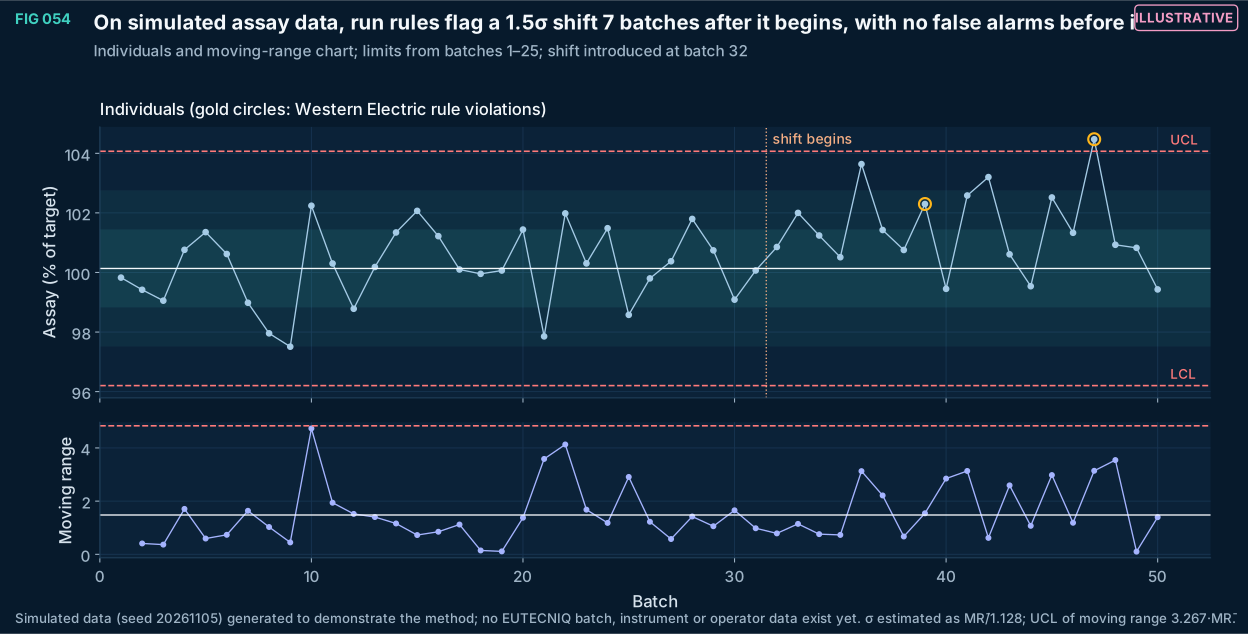
A Shewhart individuals and moving-range chart with Western Electric run rules applied to simulated assay values. Limits come from the first 25 batches; a 1.5σ upward shift starts at batch 32. Single-point 3σ limits alone react slowly to a shift of this size; the run rules catch it within a few batches.
Method, sources and limits
- Method
- I-MR chart, phase I limits from batches 1–25; Western Electric rules 1–4.
- Sources and code
- Simulated data (seed 20261105) generated to demonstrate the method; no EUTECNIQ batch, instrument or operator data exist yet. Script 09_validation_benchmarks/bench_figs.py.
- Supports
- The statistical-process-control method EUTECNIQ would apply to release and in-process data.
- Does not support
- Any statement about real batch performance.
- Limitations
- Simulated, normally distributed, independent data; real batch data are often autocorrelated or non-normal.
- Rule sets raise false-alarm rates; the choice is a policy decision.
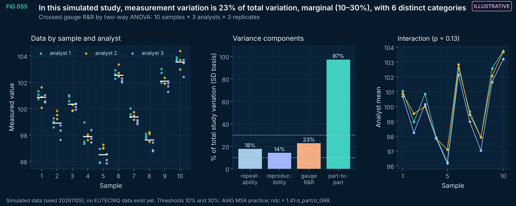
FIG 055Illustrative
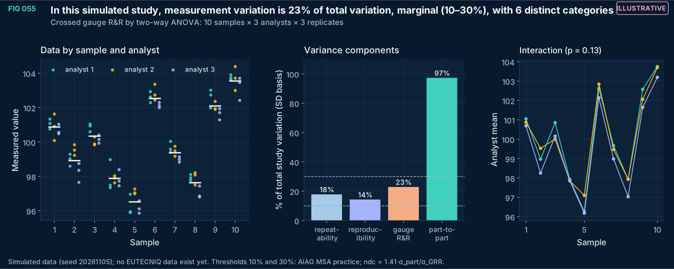
A crossed gauge repeatability and reproducibility study evaluated by two-way ANOVA with interaction on simulated data. Variance components are converted to percentages of total study variation on a standard-deviation basis, and the number of distinct categories states how many groups of samples the method can resolve.
Method, sources and limits
- Method
- Two-way random-effects ANOVA (sample, analyst, interaction) with expected-mean-square estimators truncated at zero.
- Sources and code
- Simulated data (seed 20261105) generated to demonstrate the method; no EUTECNIQ batch, instrument or operator data exist yet. Script 09_validation_benchmarks/bench_figs.py.
- Supports
- How measurement capability would be demonstrated before using a method for release decisions.
- Does not support
- Performance of any actual analytical method.
- Limitations
- Simulated data; real method validation follows ICH Q2(R2) for accuracy, precision, specificity and range.
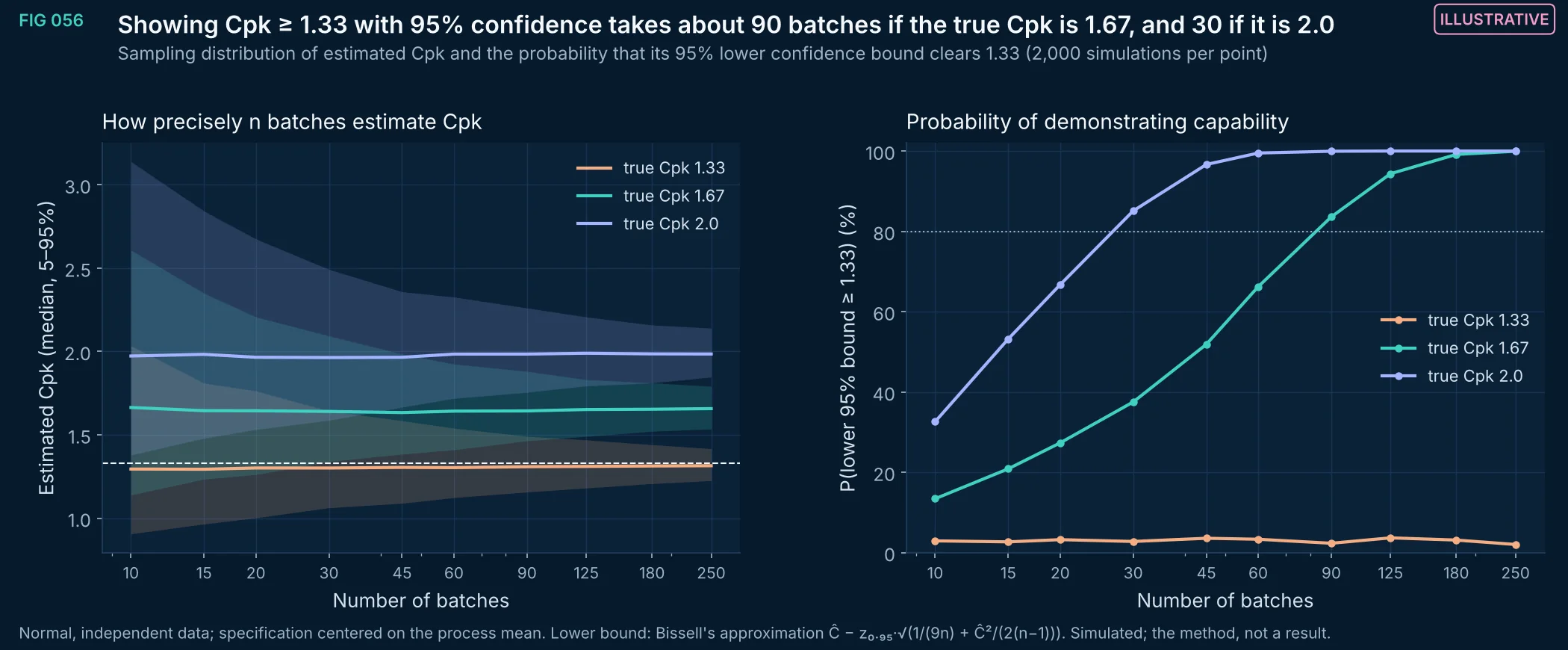
FIG 056Illustrative
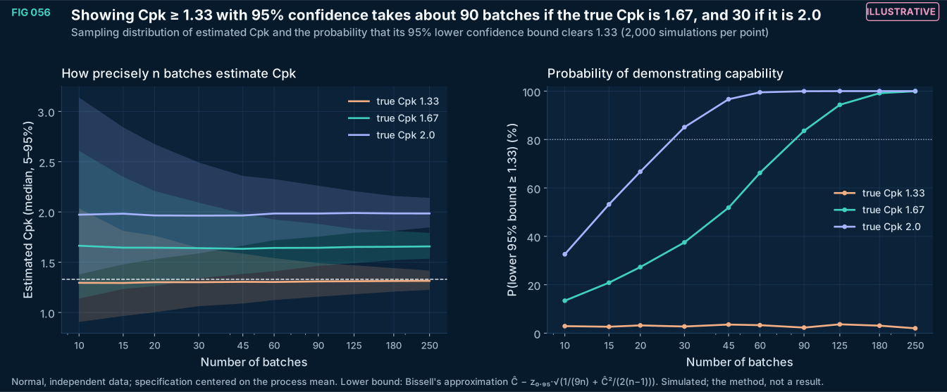
Process capability estimates are noisy at the batch counts typical of early manufacturing. Even a process with true Cpk 1.67 needs tens of batches before the 95% lower confidence bound reliably exceeds 1.33; a process sitting exactly at 1.33 essentially never demonstrates it. Capability claims should state n and the confidence bound.
Method, sources and limits
- Method
- Monte Carlo (2,000 replicates per point) of normal samples; Cpk from sample mean and SD; Bissell lower confidence bound.
- Sources and code
- Simulated data (seed 20261105) generated to demonstrate the method; no EUTECNIQ batch, instrument or operator data exist yet. Script 09_validation_benchmarks/bench_figs.py.
- Supports
- Planning how many batches a capability statement requires.
- Does not support
- Capability of any real process.
- Limitations
- Assumes normality and stability; real data need both checked first.
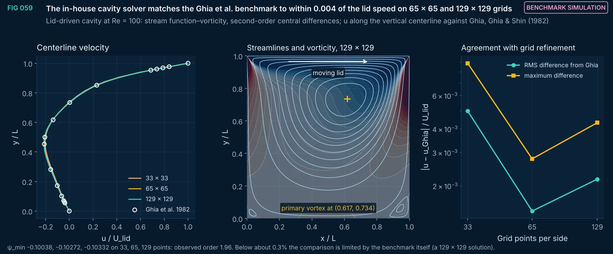
FIG 059Benchmark simulation
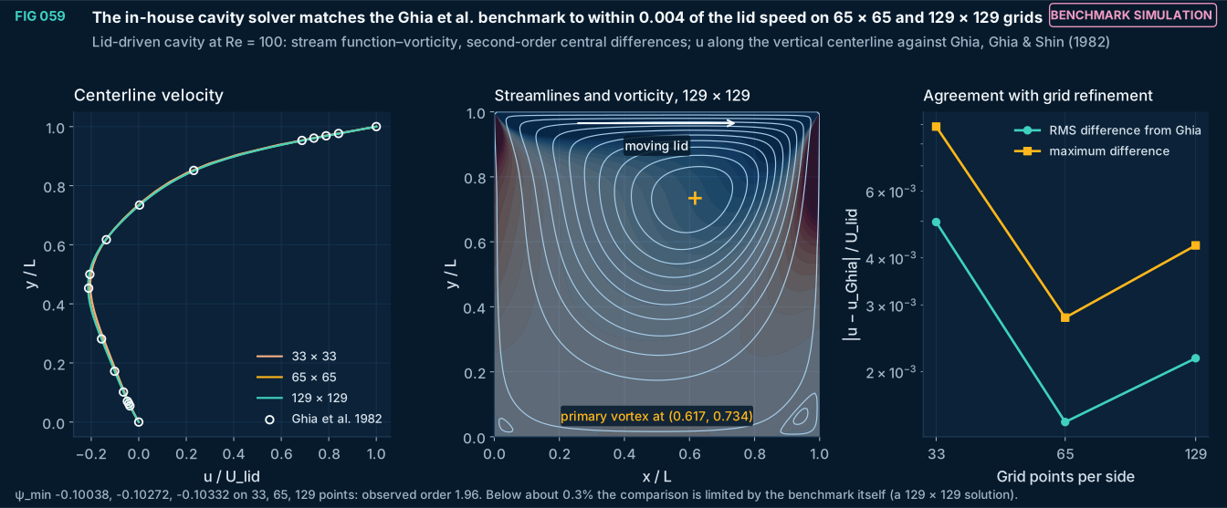
Verification of an in-house incompressible-flow solver on the lid-driven cavity at Re = 100. Centerline velocities agree with the tabulated benchmark of Ghia, Ghia and Shin (1982) to within 0.009 of the lid speed even on the coarsest grid, and the minimum stream function converges with refinement at close to the expected second order. This is the kind of check that precedes any use of a flow model for mixing or heat-transfer design.
Method, sources and limits
- Method
- Stream function–vorticity formulation, central differences, Thom wall vorticity, explicit pseudo-time marching to max |∂ω/∂t| < 10⁻⁷, sparse direct Poisson solves; Richardson-type observed order from ψ_min on three grids.
- Sources and code
- Ghia U, Ghia KN, Shin CT. J Comput Phys 1982;48(3):387–411, Table I (u-velocity, Re = 100), as transcribed in a public gist (github.com/ivan-pi). Scripts 09_validation_benchmarks/cavity.py and bench_figs.py.
- Supports
- That the numerical tools used for flow modeling reproduce a standard benchmark.
- Does not support
- Accuracy for turbulent, multiphase or three-dimensional flows.
- Limitations
- Two-dimensional, laminar, steady benchmark; industrial vessels are three-dimensional and often turbulent.
- Benchmark values from a secondary transcription of the original table.
Health information notice. These statements have not been evaluated by the Food and Drug Administration. Nothing on this site is intended to diagnose, treat, cure or prevent any disease, and nothing here is medical advice.
Read the full notice
The information is for general education only. It does not replace advice, diagnosis or treatment from a qualified health professional, or any medication a clinician has prescribed. Do not start, stop or change any medicine, supplement or herbal product because of something you read here. Talk to your doctor or pharmacist first, especially if you are pregnant or breastfeeding, have a medical condition, take any medicines, are preparing for surgery, or are caring for a child. Research findings, traditional uses and safety data are reported as their sources state them; they are not recommendations or claims about any product. If you think you may have a medical emergency, call your doctor or 911 at once.
EUTECNIQ Sciences sells no supplements or health products today and receives nothing from any product or ingredient mentioned on this site; any commercial interest it later has in an ingredient will be stated on that ingredient’s page.