

Technologies · Heat integration
Pinch analysis sets the energy target before the design
List the streams a process must heat and cool, choose the smallest temperature difference an exchanger may work across, and pinch analysis returns the least steam and cooling water that any design of that process could use. In a published four-stream example the answer is 900 kW of heating and 750 kW of cooling. This page computes it, lets you change the temperature difference, and then applies the method to a hypothetical botanical extraction plant.
Proposed capabilityEUTECNIQ has no plant and no measured stream data. The worked example uses published stream data and reproduces the published answer; the botanical plant is a hypothetical example built from the models on two other pages of this site.
Composite curves, NRCan four-stream example Temperature (°C) against cumulative heat flow (kW), minimum approach 10 K
Values in the figure
| Curve | Breakpoints (kW, °C) |
|---|---|
| Hot composite | (0, 60), (1,600, 100), (4,600, 150), (5,600, 200) |
| Cold composite | (750, 50), (1,200, 80), (5,000, 120), (6,500, 220) |
| Targets | hot utility 900 kW; cold utility 750 kW; recovered 4,850 kW; pinch 90 °C hot side, 80 °C cold side |
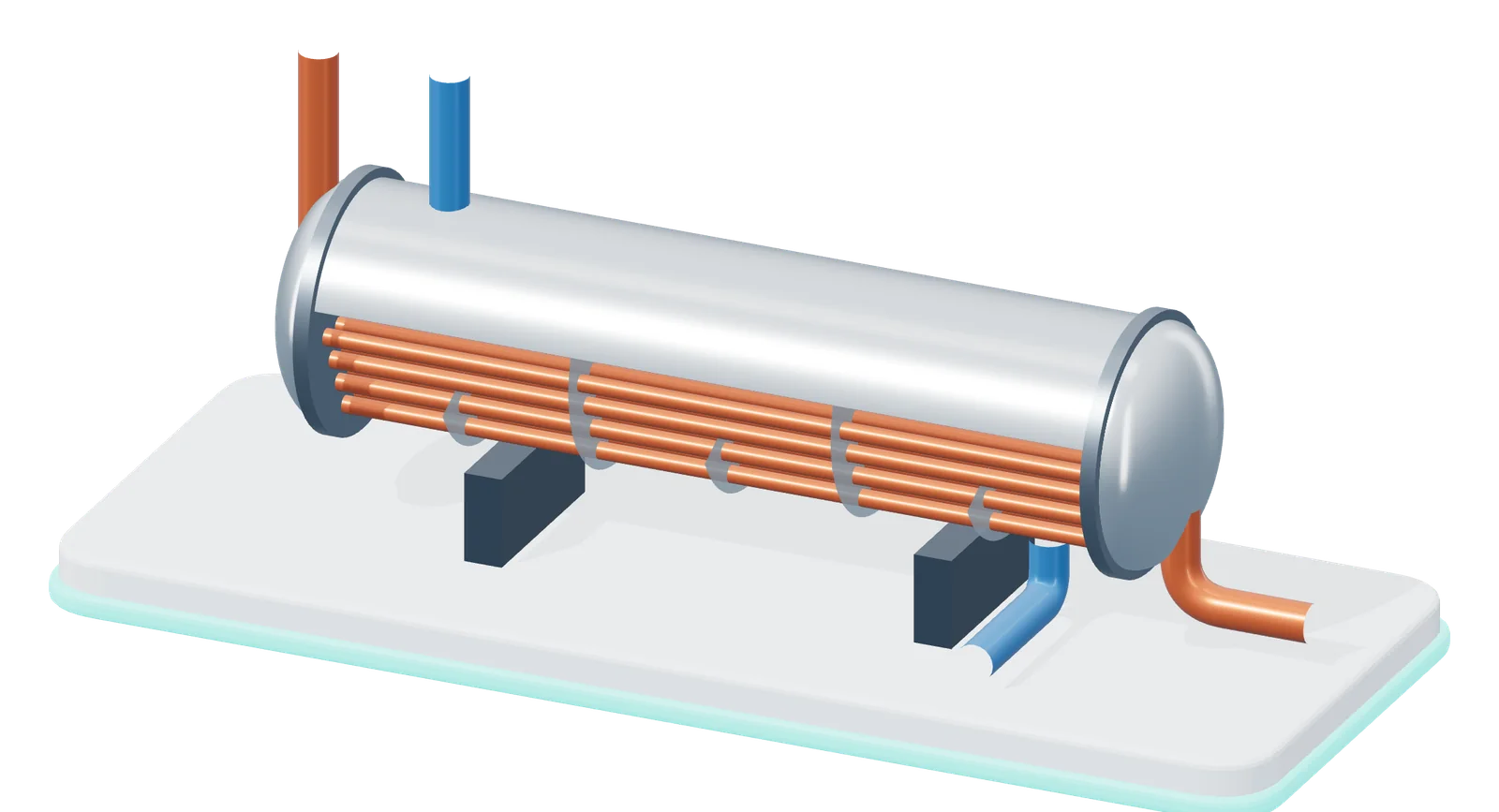
- 1 Hot stream in, through the tubes
- 2 Tube bundle
- 3 Baffles direct the shell-side flow
- 4 Cold stream in, through the shell
- 5 Cold stream out, heated
- 6 Hot stream out, cooled
Shell-and-tube heat exchanger, shell cut away, rendered by EUTECNIQ; schematic, counter-current flow.
01 · What it answers
Heat moved across the pinch is paid for twice
Hot streams must be cooled and cold streams heated. Where their temperatures allow it, one can heat the other in an exchanger, and only the remainder needs a utility (steam, hot oil, cooling water or refrigeration). Pinch analysis finds that remainder exactly, from stream data alone, before a single exchanger is chosen.
The pinch is the temperature at which the hot and cold streams come closest. It splits the process into two parts that balance independently: above it the process is a net heat sink that needs only heating, below it a net heat source that needs only cooling (NRCan 2003, pp. 26 and 38). Three rules follow (p. 38):
- No heat transfer across the pinchexcept through a heat pump, which lifts heat from below the pinch to above it.
- No cold utility above the pinchthe region above already lacks heat; cooling it adds to the steam bill.
- No hot utility below the pinchthe region below already has surplus heat; heating it adds to the cooling bill.
The penalty is exact. Every kilowatt moved across the pinch must be replaced by a kilowatt of hot utility above it and removed by a kilowatt of cold utility below it (p. 26). An existing plant that uses more than the target is breaking one of these rules somewhere, which is how pinch studies locate savings.
The heat cascade on either side of the pinch NRCan example at 10 K; α is any heat transferred across the pinch, kW
02 · Stream data and ΔTmin
Three numbers per stream are enough to set the target
Each stream that must change temperature is described by where it starts (supply temperature), where it must end (target temperature) and its heat capacity flow rate, CP, the mass flow times the specific heat (kW per kelvin). Phase changes need their latent heat as well (NRCan 2003, pp. 23 and 28). The NRCan example has two hot and two cold streams.
| Stream | Type | Supply, °C | Target, °C | CP, kW/K | Duty, kW | Shifted, °C |
|---|---|---|---|---|---|---|
| Stream 1 | hot | 200 | 100 | 20 | 2,000 | 195 → 95 |
| Stream 2 | hot | 150 | 60 | 40 | 3,600 | 145 → 55 |
| Stream 3 | cold | 80 | 120 | 80 | 3,200 | 85 → 125 |
| Stream 4 | cold | 50 | 220 | 15 | 2,550 | 55 → 225 |
Source: Natural Resources Canada (2003), Table 1, p. 23. Duty = |target − supply| × CP. Shifted temperatures are for ΔTmin = 10 K.
The smallest allowed approach
No exchanger may run with its hot and cold sides closer than ΔTmin. It is a design choice, typically 10 to 20 °C for chemical processes, 30 to 40 °C where fouling is likely or heat transfer is poor, and 3 to 5 °C for refrigeration (NRCan, p. 28).
One scale for both stream types
Hot streams are moved down by ΔTmin/2 and cold streams up by ΔTmin/2. On the shifted scale any hot stream can heat any cold stream that lies below it, and the approach is then at least ΔTmin. The shifted curves have no physical meaning of their own (NRCan, p. 31).
Describe needs, not today's equipment
Streams are what the process requires, not how the current plant happens to meet it. Do not record utility streams as process streams, and do not mix streams at different temperatures first, which can itself move heat across the pinch (NRCan, pp. 29 and 30).
03 · Problem table algorithm
The problem table finds the target with arithmetic
Linnhoff and Flower (1978) published an algebraic way to set the energy targets and locate the pinch. It needs five steps and no drawing.
- Shift every hot stream down and every cold stream up by ΔTmin/2.Hot 200 → 100 °C becomes 195 → 95 °C at ΔTmin = 10 K.
- Cut the shifted scale at every supply and target temperature.Here seven boundaries make six intervals.
- Balance each interval: (ΣCPhot − ΣCPcold) × (interval width).A positive balance is surplus heat; a negative one is a deficit.
- Cascade the surplus downward from the hottest interval, starting from zero.Heat can only flow from higher to lower temperature.
- Add the largest negative flow back at the top as hot utility.The flow is then nowhere negative; where it is zero is the pinch, and what leaves the bottom is the cold utility.
QH,min = max(0, −mink Rk), with Rk = Σi≤k (ΣCPhot − ΣCPcold)i ΔTi; QC,min = QH,min + Σhot duty − Σcold duty
Next: run it and change ΔTmin.
Steps 1 and 2 for the NRCan streams Arrows run from supply to target on the shifted scale (°C); CP in kW/K; dashed lines are the interval boundaries
04 · Worked example, computed live
At 10 K the example needs 900 kW of heating; at 20 K it needs 1,300 kW
The problem table below reproduces the published targets at 10 K. Move ΔTmin and every step is recomputed: the cascade, the targets, the composite curves and the grand composite curve. Between 1 and 40 K both utilities rise as ΔTmin rises, and the recovered heat falls by the same amount.
Composite curves Temperature (°C) against heat flow (kW); the overlap is heat recovered between streams
Grand composite curve Net heat flow (kW) through each shifted temperature (°C); zero at the pinch
The problem table at the current ΔTmin
| Interval, °C shifted | Streams present | ΣCP hot − ΣCP cold, kW/K | Interval balance, kW | Heat flowing out, kW |
|---|---|---|---|---|
| Hot utility in | – | – | – | 900 |
| 225 → 195 | 4 | -15 | -450 | 450 |
| 195 → 145 | 1, 4 | +5 | +250 | 700 |
| 145 → 125 | 1, 2, 4 | +45 | +900 | 1,600 |
| 125 → 95 | 1, 2, 3, 4 | -35 | -1,050 | 550 |
| 95 → 85 | 2, 3, 4 | -55 | -550 | 0 |
| 85 → 55 | 2, 4 | +25 | +750 | 750 |
Method, assumptions and limits
What it calculates. The minimum hot and cold utility of the NRCan four-stream example, the heat recovered between process streams, the pinch temperatures and an exchanger UA target for that recovered heat, at a minimum approach from 1 to 40 K.
Equations. Problem table algorithm as in section 03 (Linnhoff and Flower 1978). Composite curves: within each temperature interval the CPs of all streams present are added; the cold composite starts at a heat flow equal to the cold utility. UA target: vertical heat transfer between the composites over their overlap, UA = Σ ΔHk / ΔTLM,k over enthalpy intervals (area = UA/U for a uniform overall coefficient U; University of Oklahoma CHE 5480 notes).
Variables and units. Temperatures °C; CP kW/K; heat flows kW; UA kW/K.
Assumptions. Constant CP for each stream, as published; steady, continuous operation; a single ΔTmin for every match; utilities not specified (only their amounts). The UA target assumes countercurrent, vertical matching and one U for every match; it ignores the number of exchanger units, pressure drop and materials.
Valid range. ΔTmin from 1 to 40 K. Over this range the example never becomes a threshold problem (both utilities stay above zero) and the pinch stays at the inlet of stream 3, 80 °C on the cold side.
What it does not establish. A heat exchanger network, its cost or its operability. Targets are the best any network could do; designing the network is a separate step.
Verification. An independent script computes the targets by two independent routes, the problem table and a bisection that slides the cold composite until its closest approach equals ΔTmin, and they agree at every ΔTmin from 1 to 40 K. It reproduces the published 900 and 750 kW at 10 K and two further published four-stream problems: Kemp's example (20 kW hot, 60 kW cold, shifted pinch 85 °C at 10 K, as reproduced in the pina package README) and the Towler and Sinnott example (2,900 kW hot, 600 kW cold, shifted pinch 90 °C at 20 K, as reproduced on the Northwestern University Process Design Open Textbook). The on-page model was checked against 46 independently computed reference cases (926 checks, all within 10−9).
05 · Energy against capital
A smaller ΔTmin saves steam and costs exchanger area
Lowering ΔTmin lets the composite curves move closer, so more heat is recovered and less utility is bought. The price is a smaller temperature difference across every exchanger, so the network needs more area for the same duty.
In the NRCan example, going from 10 K to 5 K cuts both utilities by 200 kW and raises the UA target from 206 to 276 kW/K, 1.34 times. At 1 K the UA target is 438 kW/K. Total cost, energy plus annualized capital, therefore has a minimum at some ΔTmin (NRCan 2003, p. 27). Where it falls depends on energy prices, exchanger costs and fouling, which is why the guide gives ranges rather than one value.
Targets against ΔTmin, NRCan example Minimum utilities (kW) and the UA the recovered heat needs (kW/K); dashed line at the slider value
Values in the figure
| ΔTmin, K | Hot utility, kW | Cold utility, kW | Recovered, kW | UA, kW/K | Pinch, °C shifted |
|---|---|---|---|---|---|
| 1 | 540 | 390 | 5,210 | 437.6 | 80.5 |
| 2 | 580 | 430 | 5,170 | 368.9 | 81.0 |
| 5 | 700 | 550 | 5,050 | 275.7 | 82.5 |
| 8 | 820 | 670 | 4,930 | 228.0 | 84.0 |
| 10 | 900 | 750 | 4,850 | 205.8 | 85.0 |
| 12 | 980 | 830 | 4,770 | 188.0 | 86.0 |
| 15 | 1,100 | 950 | 4,650 | 166.7 | 87.5 |
| 20 | 1,300 | 1,150 | 4,450 | 140.3 | 90.0 |
| 25 | 1,600 | 1,450 | 4,150 | 112.6 | 92.5 |
| 30 | 1,900 | 1,750 | 3,850 | 92.3 | 95.0 |
| 35 | 2,200 | 2,050 | 3,550 | 76.2 | 97.5 |
| 40 | 2,500 | 2,350 | 3,250 | 63.2 | 100.0 |
06 · Applied to a botanical extraction plant
A second evaporator effect cuts the hypothetical plant’s minimum hot utility by 41%
An ethanol extraction plant heats its solvent and leaf, boils most of the solvent off again to recover it, condenses that vapor, and dries the extract in hot air. Built from the models on two other pages of this site, at an assumed 100 kg of dried leaf per hour, the evaporator needs 353 kW: 93% of the plant's minimum hot utility in the one-effect layout. Heat exchange alone cannot return the condenser's heat to the evaporator, because the vapor condenses below the temperature at which the liquid boils.
Hypothetical exampleNo plant, measurement or customer is behind these numbers. They show how the method would be used, from the stated assumptions below.
Streams of the one-effect layout
| Tag | Stream | Type | Temperatures, °C | Duty, kW | Basis |
|---|---|---|---|---|---|
| C1 | Extractor charge: 1,200 kg/h of 80% ethanol and 100 kg/h of leaf | cold | 20 → 70 | 50.8 | /engine/extraction/ defaults |
| C2 | Evaporator: heat the extract and boil off 864 kg/h ethanol and 216 kg/h water | cold | 70 → 80.7, boils at 80.7 | 352.6 | /engine/extraction/ recovery model; boiling point from equilibrium |
| H1 | Condenser: the same vapor condensed at 1 atm | hot | 80.7 → 79.0 | 339.3 | dew and bubble points from equilibrium |
| H2 | Condensate cooled to 20 °C for reuse | hot | 79.0 → 20 | 52.3 | CoolProp liquid enthalpies |
| C3 | Dryer inlet air: 870 kg/h | cold | 20 → 180 | 39.5 | /technologies/process-engineering/ dryer balance |
| H4 | Dryer exhaust air | hot | 85 → 50 | 9.2 | same balance; dew point 37 °C |
Assumptions
- Plant size. 100 kg/h of dried leaf, treated as continuous. A batch plant would need the time-slice treatment described in section 07.
- Extraction and recovery. The ethanol/water route of the extraction decision at its defaults: 12 kg of 80 wt% ethanol per kg of leaf, 70 °C, 90% of the solvent recovered by evaporation, recovered solvent returned at 20 °C. Charge heating 50.8 kW, evaporation 352.6 kW and condensing 339.3 kW reproduce that page's per-kilogram results within 1%.
- Boiling and condensing temperatures. From ethanol–water equilibrium (NRTL constants and the measured check of the thermodynamics page; CoolProp vapor pressures, within 0.28 K of the measured bubble points). A well-mixed evaporator whose vapor has the solvent's composition (0.610 mole fraction ethanol) boils at 80.7 °C at 1 atm and 44.2 °C at 20 kPa; the vapor condenses from 80.7 to 79.0 °C and from 44.2 to 42.7 °C. Boiling is entered as a 1 K span, as usual for constant-temperature duties.
- Spray dryer. The energy balance of process engineering at its defaults (40% solids in, 4% moisture out, air 180 °C in and 85 °C out, ambient 20 °C, 8 g/kg humidity, 5% loss) with an assumed 50 kg/h of concentrate, which implies 20 kg/h of extract solids, a 20% yield on leaf. Air 870 kg/h, heater 39.5 kW. The exhaust is cooled only to 50 °C, above its 37 °C dew point.
- Not included. Heat of mixing, heat losses from equipment, the 10% of solvent not recovered, the vacuum pump, cleaning and start-up. Utilities: steam and cooling water; their temperatures are not fixed in advance. ΔTmin 10 K for every match.
One effect at 1 atm Grand composite curve, net heat flow (kW) against shifted temperature (°C)
Two effects, 1 atm then 20 kPa Same plant; the first effect's vapor boils the second effect
Hypothetical example Computed from the assumptions above. The dashed line is 200 kPa steam, which condenses at 120.2 °C (115.2 °C shifted); only the dryer air needs heat above it.
| Evaporation layout | Hot utility, kW | Of which above 200 kPa steam, kW | Cold utility, kW | Recovered between streams, kW | Pinch, °C shifted |
|---|---|---|---|---|---|
| One effect at 1 atm | 378 | 17 | 336 | 65 | 75.7 |
| One effect at 20 kPa | 401 | 17 | 359 | 27 | 39.2 |
| Two effects, 1 atm then 20 kPa | 223 | 17 | 181 | 212 | 39.2 |
Grand composite curve points, both figures
| Layout | Points (kW, °C shifted), top to bottom |
|---|---|
| One effect at 1 atm | 377.8, 185.0; 353.5, 86.7; 10.8, 85.7; 4.4, 80.4; 4.0, 80.0; 0.0, 75.7; 141.4, 75.0; 337.6, 74.0; 336.6, 65.0; 336.1, 59.2; 335.5, 55.0; 334.6, 45.0; 334.4, 44.5; 330.9, 35.0; 329.1, 29.7; 327.3, 25.0; 335.7, 15.0 |
| Two effects, 1 atm then 20 kPa | 223.0, 185.0; 198.7, 86.7; 27.3, 85.7; 20.8, 80.4; 20.4, 80.0; 16.5, 75.7; 86.8, 75.0; 184.4, 74.0; 179.1, 65.0; 176.0, 59.2; 173.5, 55.0; 170.9, 50.2; 6.9, 49.2; 4.6, 45.0; 4.2, 44.5; 0.0, 39.2; 177.6, 37.7; 176.6, 35.0; 175.6, 32.0; 174.8, 29.7; 173.5, 26.3; 173.0, 25.0; 176.6, 20.7; 181.4, 15.0 |
Recovery is small
The process streams can exchange at most 65 kW: condenser and condensate heat for the extractor charge and the dryer air, and exhaust heat for the dryer air. Minimum hot utility is 378 kW, 353 kW of it for the evaporator.
Lower pressure does not help by itself
At 20 kPa the evaporator boils at 44 °C, but its condenser is then too cold to heat the 70 °C extractor charge, so the minimum hot utility rises to 401 kW. Changing a temperature only pays if it lets one stream serve another (the plus-minus principle, NRCan p. 37).
A temperature step creates a match
Boiling half the solvent at 1 atm and half at 20 kPa lets the first effect's vapor, condensing at 79 to 81 °C, boil the second effect at 44 °C. Minimum steam falls to 223 kW. A vapor recompressor, a heat pump placed across the pinch (NRCan p. 36), is the other route; it is not computed here.
The grand composite curve also says which steam is needed. In every layout, 200 kPa steam could supply all but 17 kW of the hot utility; that 17 kW heats the dryer air above 110 °C, which needs a hotter source such as a direct-fired or thermal-oil heater. What the numbers do not show is whether a second effect, a vacuum system or a heat pump would pay for itself. That needs equipment costs, energy prices and the plant's operating schedule.
07 · Limits
Batch plants, phase changes and real networks need more than the basic targets
Streams that do not coexist cannot exchange heat directly
A batch plant, such as the 1,000 kg batch train on the process engineering page, runs its streams at different times. Averaging every stream over the cycle (the time-average model) treats them as if they all ran at once, and can give over-optimistic targets; it equals what could be reached with maximum heat storage. The time-slice model cuts the cycle into periods in which operations are simultaneous and targets each one; heat storage is what recovers heat between periods (Becker and Maréchal 2012, citing Kemp and Macdonald 1987 and Linnhoff, Ashton and Obeng 1988).
Phase changes and mixtures bend the curves
The basic method assumes each stream's CP is constant, which fails with phase changes. Westphalen and Wolf Maciel (1999) split intervals wherever enthalpy departs from linear and reported a hot-utility target in their case study far below the constant-CP value. This page splits sensible-heat streams into pieces from reference enthalpies and takes boiling and condensing temperatures from equilibrium for the same reason.
A network still has to be designed
The targets assume ideal countercurrent matching. The number of exchangers, their area, pressure drop, materials, controllability and safety are settled in network design and process design. The area estimate from vertical heat transfer ignores the fixed cost per unit (University of Oklahoma CHE 5480 notes).
The target is only as good as the stream table
Flows, temperatures and heat capacities come from a mass and energy balance or from plant measurements. A misplaced stream, a utility recorded as a process stream, or streams mixed before analysis can move the pinch (NRCan 2003, pp. 29 and 30).
08 · Proposed use
EUTECNIQ would set energy targets while the process is still on paper
The cheapest time to change a pressure, a temperature or the number of evaporator effects is before equipment is bought. EUTECNIQ proposes to run pinch analysis on every extraction, concentration and drying process it designs or transfers, alongside the mass and energy balance.
Proposed capabilityNone of this has been carried out. EUTECNIQ is in formation and has no plant, data or clients.
- Stream table from the balance.Supply and target temperatures, flows and heat capacities taken from the process mass and energy balance, with phase changes from reference property data.
- Targets and the grand composite.Minimum steam and cooling water, the pinch, and which steam or heat-transfer fluid levels are needed, over a range of ΔTmin.
- Process changes before equipment.Evaporator pressure and number of effects, vapor recompression, extraction temperature and solvent ratio screened against the targets, with the extraction decision for the solvent route itself.
- Batch schedules.Time-slice targets and the heat storage needed to connect periods, where the plant runs in batches.
- Hand-offs.Exergy analysis to locate where the potential to do work is lost, and process CFD for exchangers, dryers and vessels whose detail the targets cannot see.
Proposed deliverables: a stream table with its sources, composite and grand composite curves, utility targets against ΔTmin, a list of process changes ranked by their effect on the targets, and the assumptions that would have to hold for each.
09 · Sources
References opened for this page
- Natural Resources Canada, CanmetENERGY. Pinch Analysis: For the Efficient Use of Energy, Water & Hydrogen. 2003. ISBN 0-662-34964-4, Cat. M39-96/2003E. Table 1 (p. 23) and targets (p. 25) of the worked example; pinch and penalty (pp. 25–26); ΔTmin ranges and trade-off (pp. 26–28); data extraction (pp. 28–30); grand composite curve and shifted curves (pp. 30–32); heat pumps (p. 36); plus-minus principle (p. 37); the three rules (p. 38). natural-resources.canada.ca
- Linnhoff B, Flower JR. Synthesis of heat exchanger networks: I. Systematic generation of energy optimal networks. AIChE J. 1978;24(4):633–642. doi.org/10.1002/aic.690240411 (bibliographic record checked; credited with the algebraic targeting method by Westphalen and Wolf Maciel 1999)
- Westphalen DL, Wolf Maciel MR. Pinch analysis based on rigorous physical properties. Braz J Chem Eng. September 1999. scielo.br
- Becker H, Maréchal F. Targeting industrial heat pump integration in multi-period problems. In: Karimi IA, Srinivasan R, eds. Proceedings of the 11th International Symposium on Process Systems Engineering (PSE 2012), Singapore. Elsevier; 2012. infoscience.epfl.ch (time-average and time-slice models; heat storage)
- University of Oklahoma, CHE 5480 course notes. Pinch Analysis Part 3: Units and Area Targeting, Supertargeting. ou.edu (vertical heat transfer, A = Q/(U ΔTLM) per interval)
- Verification case: pina, pinch analysis package for Python, README "Basic example" (MIT license), data attributed to Kemp IC, Pinch Analysis and Process Integration, 2nd ed., p. 4. github.com/FitzOReilly/pina
- Verification case: Zuckerman M. Pinch analysis. Northwestern University Process Design Open Textbook; 2015 (example data attributed to Towler G, Sinnott R. Chemical Engineering Design, 2nd ed., 2013). processdesign.mccormick.northwestern.edu
- Lai H-S, Lin Y-F, Tu C-H. Isobaric (vapor + liquid) equilibria for the ternary system of (ethanol + water + 1,3-propanediol) and three constituent binary systems at P = 101.3 kPa. J Chem Thermodyn. 2014;68:13–19. doi.org/10.1016/j.jct.2013.08.020 (measured bubble points used as a check, as tabulated on /insights/thermodynamics/)
- Renon H, Prausnitz JM. Local compositions in thermodynamic excess functions for liquid mixtures. AIChE J. 1968;14(1):135–144. doi.org/10.1002/aic.690140124; constants from Kooijman HA, Taylor R, ChemSep NRTL file "DECHEMA NRTL data @ 1 atm" (2008), as used on /insights/thermodynamics/. chemsep.org
- Bell IH, Wronski J, Quoilin S, Lemort V. Pure and pseudo-pure fluid thermophysical property evaluation and the open-source thermophysical property library CoolProp. Ind Eng Chem Res. 2014;53(6):2498–2508. doi.org/10.1021/ie4033999 (CoolProp 8.0.0 used)
- ASHRAE Handbook—Fundamentals (SI). Atlanta: ASHRAE; 2017. Chapter 1, Psychrometrics (moist-air enthalpy, as in the spray-dryer balance of /technologies/process-engineering/).
Health information notice. These statements have not been evaluated by the Food and Drug Administration. Nothing on this site is intended to diagnose, treat, cure or prevent any disease, and nothing here is medical advice.
Read the full notice
The information is for general education only. It does not replace advice, diagnosis or treatment from a qualified health professional, or any medication a clinician has prescribed. Do not start, stop or change any medicine, supplement or herbal product because of something you read here. Talk to your doctor or pharmacist first, especially if you are pregnant or breastfeeding, have a medical condition, take any medicines, are preparing for surgery, or are caring for a child. Research findings, traditional uses and safety data are reported as their sources state them; they are not recommendations or claims about any product. If you think you may have a medical emergency, call your doctor or 911 at once.
EUTECNIQ Sciences sells no supplements or health products today and receives nothing from any product or ingredient mentioned on this site; any commercial interest it later has in an ingredient will be stated on that ingredient’s page.