

Three phase diagrams set solvent recovery, partitioning and crystallization, and each can be computed before a pilot run
Every curve comes from a published model with declared parameters, laid over measured data, misses included. EUTECNIQ would compute these before choosing solvents; nothing here is EUTECNIQ data.
The COSMO-SAC curves here come from an open variant of COSMO-RS
Explanation, details and sources
This page reports no COSMO-RS results; its COSMO-SAC curves use our own density-functional surfaces from the quantum chemistry page.
COSMO-RS (conductor-like screening model for real solvents) was introduced by Klamt in 1995 and refined and parameterized in 1998. It combines a quantum-chemistry calculation of each molecule in a perfect conductor with statistical thermodynamics of interacting surface segments, and needs no experimental mixture data (Eckert & Klamt 2002). Its commercial implementation is BIOVIA COSMOtherm (Dassault Systèmes), which reads one COSMO file per compound.
COSMO-SAC (segment activity coefficient) was proposed by Lin and Sandler in 2002 as an activity-coefficient model based on COSMO-RS: the same screening charges, with each molecule treated as a collection of surface segments whose activity coefficients sum to the molecule's. It needs one radius per atom and three universal parameters. The 2010 revision (Hsieh, Sandler & Lin) uses separate σ-profiles for different hydrogen-bonding groups and a temperature-dependent electrostatic term.
Why COSMO-SAC here: its equations, universal constants and a benchmark open-source implementation (NIST; Bell et al. 2020, MIT license) are published, so every number can be checked line by line and regenerated. Our surfaces use the COSMO-RS atomic radii (Klamt et al. 1998) and open-source PySCF; the COSMO-SAC constants were fitted to surfaces from a different quantum-chemistry setup, so the results are a screening-level ranking.
The surfaces, σ-profiles and the COSMO-SAC code are documented, with every run archived, on Quantum chemistry.
Six molecules, three phase diagrams and every curve laid over published measurements
Solids (SLE)
Solvents
Water
- Formula
- H₂O
- Molar mass
- 18.015 g/mol
- PubChem CID
- 962
- On this page
- VLE, LLE, SLE solvent
- COSMO surface
- 43 Ų
Ethanol
- Formula
- C₂H₆O
- Molar mass
- 46.07 g/mol
- PubChem CID
- 702
- On this page
- VLE, LLE, SLE solvent
- COSMO surface
- 89 Ų
Ethyl acetate
- Formula
- C₄H₈O₂
- Molar mass
- 88.11 g/mol
- PubChem CID
- 8857
- On this page
- LLE, SLE solvent
- COSMO surface
- 137 Ų
Salicylic acid
- Formula
- C₇H₆O₃
- Molar mass
- 138.12 g/mol
- PubChem CID
- 338
- On this page
- SLE solute; crystallization
- COSMO surface
- 161 Ų
Caffeine
- Formula
- C₈H₁₀N₄O₂
- Molar mass
- 194.19 g/mol
- PubChem CID
- 2519
- On this page
- SLE solute
- COSMO surface
- 217 Ų
Vanillin
- Formula
- C₈H₈O₃
- Molar mass
- 152.15 g/mol
- PubChem CID
- 1183
- On this page
- SLE solute
- COSMO surface
- 186 Ų
Data table: the six molecules
| Molecule | Formula | PubChem CID | Molar mass (g/mol) | Role on this page | Atoms | COSMO surface (Ų) |
|---|---|---|---|---|---|---|
| Water | H₂O | 962 | 18.015 | VLE, LLE, SLE solvent | 3 | 43.1 |
| Ethanol | C₂H₆O | 702 | 46.07 | VLE, LLE, SLE solvent | 9 | 88.9 |
| Ethyl acetate | C₄H₈O₂ | 8857 | 88.11 | LLE, SLE solvent | 14 | 137.2 |
| Salicylic acid | C₇H₆O₃ | 338 | 138.12 | SLE solute; crystallization | 16 | 160.9 |
| Caffeine | C₈H₁₀N₄O₂ | 2519 | 194.19 | SLE solute | 24 | 217.1 |
| Vanillin | C₈H₈O₃ | 1183 | 152.15 | SLE solute | 19 | 186.0 |
Key. Points are published measurements; solid lines are fitted correlations; dashed and dotted lines are predictions that saw no mixture data.
- Fitted curve≠independent prediction
- Theoretical stage≠a real tray or packing height
- Equilibrium yield≠the yield of a real, finite-time crystallizer
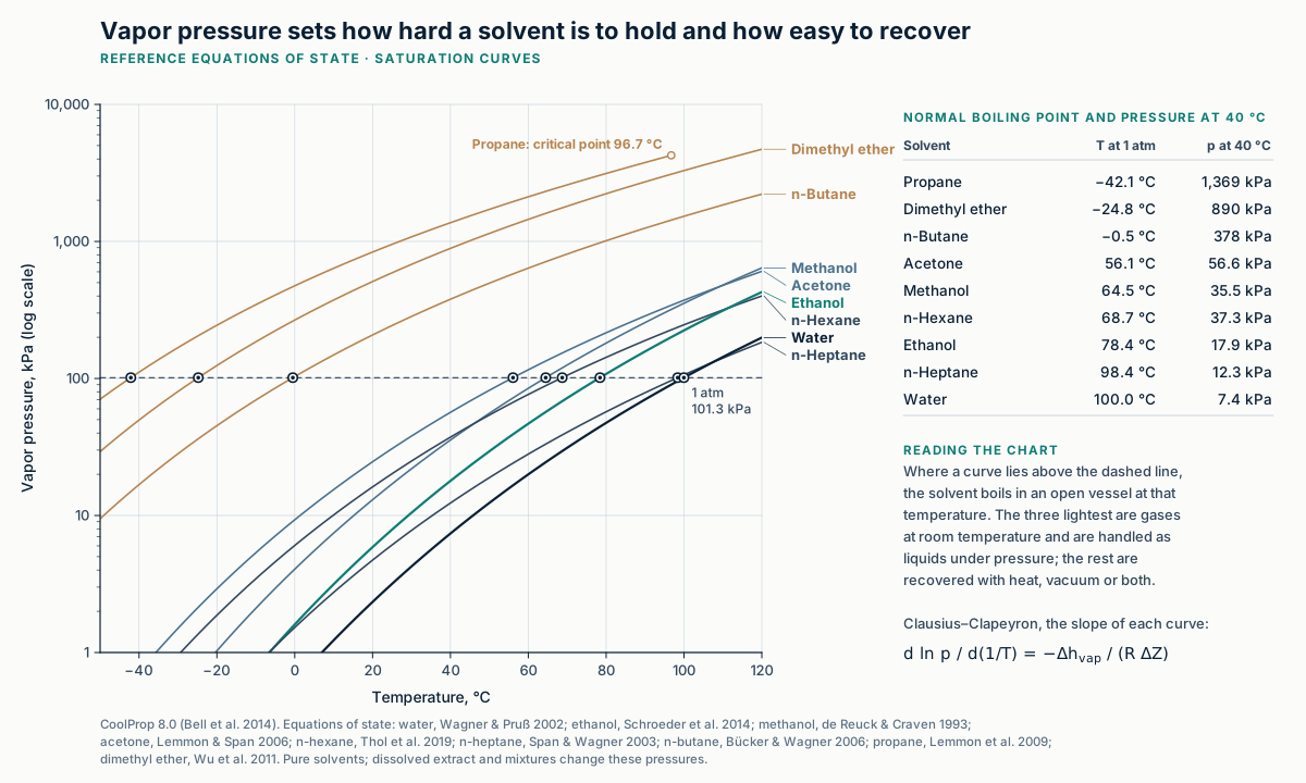
Three diagrams, three plant decisions
The models trade measured data for computation
Model reference table: what each model needs, where it works and its source
| Model | Key relation | Needs | Works well for, and limits | On this page |
|---|---|---|---|---|
| Raoult's law (Raoult 1887) | yiP = xiPisat; every γi = 1 | Each pure liquid's vapor pressure; nothing about the mixture | Chemically similar molecules. For ethanol–water it predicts no azeotrope. | VLE, as the ideal reference |
| Margules (1895), van Laar (1910) | GE/RT = x1x2(A21x1 + A12x2); van Laar: A12A21x1x2/(A12x1 + A21x2) | One or two constants per pair, fitted to mixture data | Simple binary mixtures over a narrow range; empirical. | Not used |
| Wilson (1964) | GE/RT = −Σi xi ln Σj xjΛij | Two energy constants per pair plus liquid molar volumes | Fully miscible polar mixtures such as alcohol–water. Cannot represent two liquid layers. | Not used |
| NRTL (Renon & Prausnitz 1968) | Gij = exp(−αijτij), τij = aij + bij/T | Three constants per pair: two energies and a non-randomness α | Vapor–liquid and liquid–liquid equilibria. Constants fitted to one kind of data can fail for the other (LLE tab). | VLE, McCabe–Thiele, LLE |
| UNIQUAC (Abrams & Prausnitz 1975) | ln γi = ln γiC + ln γiR | Each molecule's size r and surface area q, plus two energies per pair | Partly or fully miscible mixtures of molecules of very different size. | Not used directly; UNIFAC builds on it |
| UNIFAC (Fredenslund et al. 1975) | ln γiR = Σk νk(ln Γk − ln Γk(i)) | Only the molecule's functional groups | Mixtures never measured, provided every group is in the parameter table. | Not used in its original form |
| Modified UNIFAC, Dortmund (Weidlich & Gmehling 1987) | Ψnm = exp[−(a + bT + cT²)/T] | Groups; interactions vary with temperature | Vapor–liquid equilibrium and solubility with temperature-dependent group interactions. | VLE and SLE (DDBST published parameters) |
| UNIFAC-LLE (Magnussen et al. 1981) | Same form, separate parameter table | Groups; parameters fitted to liquid–liquid data | Predicting liquid splitting. | LLE |
| COSMO-RS (Klamt 1995) | μi = μiC + ∫ pi(σ) μS(σ) dσ | A quantum-chemistry calculation of each molecule's surface charge σ; no mixture data | New molecules such as natural products; results must be checked against data for each new compound class. | Background for the Quantum chemistry page |
| COSMO-SAC (Lin & Sandler 2002) | ln γi = ni Σσ pi(σ)[ln ΓS(σ) − ln Γi(σ)] + ln γiSG | The same σ-profiles, in an openly published formulation | Screening-level activity coefficients from structure alone. | Computed on the Quantum chemistry page |
| Peng–Robinson (1976) | P = RT/(v − b) − a(T)/[v(v + b) + b(v − b)] | Critical temperature, pressure and acentric factor; one kij per pair | Gases, hydrocarbons and CO₂ at high pressure; liquid densities and strongly polar mixtures less accurate. | Background for supercritical CO₂ on Extraction |
| PC-SAFT (Gross & Sadowski 2001) | Ares = Ahc + Adisp | Three constants per molecule: segment number m, size σ, energy ε/k | Chain molecules, polymers and high pressure. | Not used |
Explanation, details and sources
Left-hand models need measured data for every liquid pair; right-hand models predict from structure and still need checking. A phase diagram maps which phases (vapor, liquid layers, solid) exist at each temperature and composition. Each one on this page is drawn from real data. Most of the models estimate an activity coefficient: how far a molecule departs from ideal behavior in a mixture. Equations of state describe a whole fluid at any pressure.
Why it mattersA botanical extract holds hundreds of compounds never measured in mixtures, so predictive models would screen solvents and measurements would confirm the short list. Related: COSMO-SAC calculations in Quantum chemistry · supercritical CO₂ in Extraction
Ethanol and water boil together at 95.4 wt% ethanol
Both non-ideal models place the azeotrope within 0.01 mole fraction and 0.12 °C of the measurement; the ideal model misses it.
Show data: measured points and model values at the same compositions
| x ethanol (liquid) | T measured, °C | T NRTL | T UNIFAC | T Raoult | y ethanol measured | y NRTL | y UNIFAC |
|---|---|---|---|---|---|---|---|
| 0.000 | 100.00 | 100.00 | 100.00 | 100.00 | 0.000 | 0.000 | 0.000 |
| 0.015 | 96.12 | 96.36 | 95.81 | 99.49 | 0.139 | 0.136 | 0.153 |
| 0.035 | 92.46 | 92.78 | 92.14 | 98.83 | 0.261 | 0.256 | 0.273 |
| 0.100 | 86.64 | 86.50 | 86.33 | 96.77 | 0.436 | 0.442 | 0.443 |
| 0.183 | 83.51 | 83.25 | 83.45 | 94.36 | 0.525 | 0.531 | 0.524 |
| 0.292 | 81.73 | 81.40 | 81.69 | 91.50 | 0.585 | 0.586 | 0.578 |
| 0.394 | 80.74 | 80.39 | 80.65 | 89.09 | 0.611 | 0.622 | 0.617 |
| 0.501 | 79.91 | 79.58 | 79.79 | 86.79 | 0.648 | 0.660 | 0.659 |
| 0.543 | 79.58 | 79.30 | 79.49 | 85.94 | 0.669 | 0.677 | 0.676 |
| 0.631 | 78.89 | 78.78 | 78.95 | 84.26 | 0.714 | 0.716 | 0.718 |
| 0.749 | 78.52 | 78.28 | 78.40 | 82.17 | 0.781 | 0.783 | 0.786 |
| 0.794 | 78.49 | 78.16 | 78.27 | 81.42 | 0.814 | 0.813 | 0.816 |
| 0.848 | 78.25 | 78.07 | 78.16 | 80.55 | 0.855 | 0.854 | 0.856 |
| 0.899 | 78.18 | 78.06 | 78.12 | 79.76 | 0.898 | 0.897 | 0.899 |
| 0.949 | 78.22 | 78.13 | 78.16 | 79.01 | 0.946 | 0.945 | 0.946 |
| 1.000 | 78.30 | 78.28 | 78.28 | 78.28 | 1.000 | 1.000 | 1.000 |
Model bubble temperatures and vapor compositions computed at each measured liquid composition (compute/tables.py), not read off the plotted curves. The measured endpoints (x = 0 and 1) are pure-liquid boiling points.
Each McCabe–Thiele step is one equilibrium stage
bottom: from (xB, xB) to the feed line
Assumptions
- Equilibrium curve: NRTL with the parameters validated above, 101.3 kPa
- Constant molar overflow (equal molar heats of vaporization); an approximation for ethanol–water
- Saturated-liquid feed (q = 1), total condenser, partial reboiler counted as a stage
- Theoretical stages: real trays or packing need an efficiency factor measured at pilot scale
- Slider values are examples, not EUTECNIQ data
Method, assumptions and limits
- What it calculates
- The number of ideal equilibrium stages, the feed stage, the minimum and actual reflux ratios, the ethanol recovery and the vapor boil-up for a continuous column that concentrates an ethanol–water feed at 101.3 kPa.
- Equations
- Equilibrium y*(x) from NRTL bubble points (dense precomputed grid, linear interpolation). Rectifying line y = R/(R + 1)·x + xD/(R + 1). Feed line x = zF (q = 1). Stripping line through (xB, xB) and the intersection of the other two. Minimum reflux from the steepest line through (xD, xD) that touches the equilibrium curve between zF and xD (tangent pinch): Rmin = s/(1 − s). Overall balances: D/F = (zF − xB)/(xD − xB); recovery = xDD/(zFF); vapor per mole distillate = R + 1. Stages stepped from the top; the last stage is counted as a fraction.
- Variables and units
- Slider inputs in weight percent ethanol, converted to mole fractions with 46.07 and 18.02 g/mol; R dimensionless; recovery in percent of the ethanol fed.
- Assumptions
- Constant molar overflow; saturated-liquid feed; total condenser; partial reboiler counted as one stage; ideal (100% efficient) stages; no heat losses; pressure drop ignored.
- Valid range
- Feed 5–60 wt%, distillate 60–94 wt% (below the NRTL azeotrope at 95.0 wt%; the measured azeotrope is at 95.4 wt%), bottoms 0.1–2 wt%, reflux 1.05–3 times minimum. Near 94 wt% the stage count becomes very sensitive to the equilibrium model; above 150 stages the page reports "more than 150".
- What it does not establish
- Real tray counts or packing heights (these need efficiencies measured at pilot scale), column diameter, energy cost, or the effect of other extract components on the equilibrium.
- References
- McCabe & Thiele 1925; Renon & Prausnitz 1968; parameters as in the VLE figure.
- Verification
- An independent Python implementation (tests/numerics/ref/insights-thermodynamics.py) recomputes the equilibrium with the thermo package's own NRTL class and steps the stages with exact root-finding; the page agrees within the tolerances listed in Methods, data and checks below.
90 wt% ethanol needs 18.0 theoretical stages at reflux 1.03; 94 wt% needs 36.7 stages at reflux 3.22 (same multiple of minimum reflux).
Explanation, details and sources
The McCabe–Thiele method (1925) counts the stages a column needs for a feed strength, purity targets and reflux (the share of condensed vapor sent back down). Steps crowd where the curve nears the diagonal.
Why it mattersExtraction ethanol is reused only after recovery. Stage count sets column height, and the reflux ratio sets steam use, because the vapor boiled up equals (R + 1) times the distillate. Related: solvent recovery in Process engineering
Water and ethyl acetate form two liquid layers
Mole percent. Hover a tie line, or choose a measured one from the list.
Fitted NRTL follows the measured tie lines within 0.02 mole fraction; the two layers merge near 18 mol% ethanol.
Show data: measured tie lines and each model's tie line at the same ethanol level (mol%)
| Tie line and source | Water layer: water | ethanol | ethyl acetate | Ester layer: water | ethanol | ethyl acetate | K ethanol |
|---|---|---|---|---|---|---|---|
| Tie line 1, measured | 96.8 | 0.0 | 3.2 | 14.2 | 0.0 | 85.8 | — |
| NRTL fitted to these data | 98.3 | 0.0 | 1.7 | 17.7 | 0.0 | 82.3 | — |
| UNIFAC-LLE, prediction | 99.5 | 0.0 | 0.5 | 12.7 | 0.0 | 87.3 | — |
| NRTL, vapor–liquid parameters, prediction | 91.7 | 0.0 | 8.3 | 50.6 | 0.0 | 49.4 | — |
| Tie line 2, measured | 96.3 | 1.0 | 2.7 | 15.7 | 1.8 | 82.5 | 1.80 |
| NRTL fitted to these data | 97.1 | 1.0 | 1.9 | 19.4 | 2.2 | 78.4 | 2.16 |
| UNIFAC-LLE, prediction | 98.3 | 1.0 | 0.7 | 16.6 | 4.6 | 78.8 | 4.58 |
| NRTL, vapor–liquid parameters, prediction | 90.0 | 1.0 | 9.0 | 53.5 | 2.2 | 44.3 | 2.16 |
| Tie line 3, measured | 94.5 | 2.6 | 2.9 | 17.0 | 4.2 | 78.8 | 1.62 |
| NRTL fitted to these data | 95.1 | 2.6 | 2.3 | 22.4 | 5.5 | 72.2 | 2.10 |
| UNIFAC-LLE, prediction | 96.4 | 2.6 | 1.0 | 26.7 | 12.1 | 61.2 | 4.64 |
| NRTL, vapor–liquid parameters, prediction | 87.1 | 2.6 | 10.3 | 58.0 | 4.9 | 37.2 | 1.87 |
| Tie line 4, measured | 92.7 | 4.0 | 3.3 | 19.6 | 6.8 | 73.6 | 1.70 |
| NRTL fitted to these data | 93.3 | 4.0 | 2.7 | 25.2 | 8.2 | 66.6 | 2.05 |
| UNIFAC-LLE, prediction | 94.7 | 4.0 | 1.3 | 41.6 | 17.9 | 40.5 | 4.48 |
| NRTL, vapor–liquid parameters, prediction | 84.2 | 4.0 | 11.8 | 61.9 | 6.5 | 31.6 | 1.63 |
| Tie line 5, measured | 90.6 | 6.1 | 3.3 | 23.1 | 10.2 | 66.7 | 1.67 |
| NRTL fitted to these data | 90.4 | 6.1 | 3.5 | 29.8 | 11.9 | 58.3 | 1.95 |
| UNIFAC-LLE, prediction | 92.2 | 6.1 | 1.7 | 58.0 | 20.5 | 21.5 | 3.36 |
| NRTL, vapor–liquid parameters, prediction | no second liquid layer predicted at this ethanol level | ||||||
| Tie line 6, measured | 87.6 | 8.0 | 4.4 | 29.5 | 13.5 | 57.0 | 1.69 |
| NRTL fitted to these data | 87.7 | 8.0 | 4.3 | 34.5 | 14.8 | 50.8 | 1.84 |
| UNIFAC-LLE, prediction | 89.8 | 8.0 | 2.2 | 65.8 | 20.1 | 14.1 | 2.51 |
| NRTL, vapor–liquid parameters, prediction | no second liquid layer predicted at this ethanol level | ||||||
| Tie line 7, measured | 85.2 | 9.5 | 5.3 | 34.5 | 15.9 | 49.6 | 1.67 |
| NRTL fitted to these data | 85.4 | 9.5 | 5.1 | 38.4 | 16.6 | 45.0 | 1.75 |
| UNIFAC-LLE, prediction | 87.9 | 9.5 | 2.6 | 70.1 | 19.2 | 10.7 | 2.02 |
| NRTL, vapor–liquid parameters, prediction | no second liquid layer predicted at this ethanol level | ||||||
| Tie line 8, measured | 83.3 | 10.7 | 6.0 | 40.7 | 17.4 | 41.9 | 1.63 |
| NRTL fitted to these data | 83.4 | 10.7 | 5.9 | 41.6 | 17.8 | 40.6 | 1.66 |
| UNIFAC-LLE, prediction | 86.3 | 10.7 | 3.0 | 73.0 | 18.2 | 8.8 | 1.70 |
| NRTL, vapor–liquid parameters, prediction | no second liquid layer predicted at this ethanol level | ||||||
Model tie lines solved at the measured ethanol fraction of the water layer (compute/tables.py). K = ethanol mole fraction in the ester layer ÷ that in the water layer. Mean absolute errors in the summary above are taken over these compositions.
Two layers form where the free-energy surface folds
Data table: surface values along the water–ethyl acetate edge and the tie-line ends
| x ethyl acetate | ΔGmix/RT | Local stability |
|---|---|---|
| 0.0 | 0.000 | stable or metastable |
| 0.1 | 0.019 | unstable (inside the spinodal) |
| 0.2 | 0.058 | unstable (inside the spinodal) |
| 0.3 | 0.065 | unstable (inside the spinodal) |
| 0.4 | 0.044 | unstable (inside the spinodal) |
| 0.5 | 0.005 | unstable (inside the spinodal) |
| 0.6 | −0.042 | stable or metastable |
| 0.7 | −0.090 | stable or metastable |
| 0.8 | −0.124 | stable or metastable |
| 0.9 | −0.123 | stable or metastable |
| 1.0 | 0.000 | stable or metastable |
| Water layer: x ethanol | x ethyl acetate | ΔGmix/RT | Ester layer: x ethanol | x ethyl acetate | ΔGmix/RT |
|---|---|---|---|---|---|
| 0.000 | 0.032 | −0.015 | 0.000 | 0.858 | −0.130 |
| 0.010 | 0.027 | −0.065 | 0.018 | 0.825 | −0.215 |
| 0.026 | 0.029 | −0.119 | 0.042 | 0.788 | −0.294 |
| 0.040 | 0.033 | −0.159 | 0.068 | 0.736 | −0.363 |
| 0.061 | 0.033 | −0.211 | 0.102 | 0.667 | −0.440 |
| 0.080 | 0.044 | −0.256 | 0.135 | 0.570 | −0.498 |
| 0.095 | 0.053 | −0.290 | 0.159 | 0.496 | −0.534 |
| 0.107 | 0.060 | −0.317 | 0.174 | 0.419 | −0.546 |
Each model tie line is a common tangent: its chord runs below the surface, so two layers have the lower Gibbs energy.
Warming pushes ethyl acetate out of water
Show data: mutual solubility, measured and modeled (mol%)
| T, °C | Ester in water, measured | fitted NRTL | UNIFAC-LLE | vapor NRTL | Water in ester, measured | fitted NRTL | UNIFAC-LLE | vapor NRTL |
|---|---|---|---|---|---|---|---|---|
| 25 | 1.63 | 1.75 | 0.52 | 7.65 | 17.33 | 16.66 | 12.22 | 50.70 |
| 30 | 1.55 | 1.66 | 0.55 | 8.26 | 18.85 | 17.74 | 12.70 | 50.61 |
| 35 | 1.49 | 1.58 | 0.58 | 8.91 | 19.97 | 18.85 | 13.17 | 50.61 |
| 40 | 1.44 | 1.51 | 0.61 | 9.61 | 21.11 | 19.99 | 13.65 | 50.71 |
| 45 | 1.40 | 1.45 | 0.64 | 10.36 | 21.79 | 21.14 | 14.13 | 50.92 |
| 50 | 1.37 | 1.39 | 0.68 | 11.17 | 22.59 | 22.31 | 14.61 | 51.24 |
| 55 | 1.34 | 1.34 | 0.71 | 12.05 | 23.33 | 23.49 | 15.09 | 51.69 |
| 60 | 1.33 | 1.29 | 0.74 | 13.00 | 24.14 | 24.68 | 15.58 | 52.28 |
Measured: Grande & Marschoff 2005. Ester is ethyl acetate.
Only the fitted model follows both measured trends; the vapor-fitted NRTL predicts an ester layer that is half water.
Explanation, details and sources
Why it mattersLiquid–liquid extraction moves target compounds into one layer and leaves sugars and salts in the other; ester dissolved in the water layer is lost unless stripped. The same calculation with a compound's own activity coefficients gives its partition ratio; that is where COSMO-type models come in.
The solvent moves solubility by orders of magnitude
The dark dotted line is ideal solubility: it needs only the melting point and heat of melting and ignores the solvent. Points are measurements; dashed lines are UNIFAC predictions.
Ideal solubility is 167× too high in water and 3.1× too low in ethanol; UNIFAC narrows this to 11-fold and 1.5-fold. Ethanol dissolves 524× more than water.
Show data: every measured point with the ideal and UNIFAC values at the same temperature
| Compound | Solvent | Study | T, °C | x measured | x ideal | x UNIFAC |
|---|---|---|---|---|---|---|
| Salicylic acid | water | Nordström 2006 | 9.95 | 1.60 × 10⁻⁴ | 0.0273 | 1.74 × 10⁻³ |
| Salicylic acid | water | Nordström 2006 | 15.00 | 1.80 × 10⁻⁴ | 0.0327 | 2.10 × 10⁻³ |
| Salicylic acid | water | Nordström 2006 | 20.00 | 2.10 × 10⁻⁴ | 0.0390 | 2.54 × 10⁻³ |
| Salicylic acid | water | Nordström 2006 | 25.00 | 2.50 × 10⁻⁴ | 0.0462 | 3.06 × 10⁻³ |
| Salicylic acid | water | Nordström 2006 | 30.00 | 3.00 × 10⁻⁴ | 0.0544 | 3.69 × 10⁻³ |
| Salicylic acid | water | Nordström 2006 | 35.00 | 3.70 × 10⁻⁴ | 0.0638 | 4.46 × 10⁻³ |
| Salicylic acid | water | Nordström 2006 | 40.00 | 4.50 × 10⁻⁴ | 0.0743 | 5.39 × 10⁻³ |
| Salicylic acid | water | Nordström 2006 | 45.00 | 5.50 × 10⁻⁴ | 0.0862 | 6.55 × 10⁻³ |
| Salicylic acid | water | Nordström 2006 | 50.00 | 6.80 × 10⁻⁴ | 0.0996 | 7.98 × 10⁻³ |
| Salicylic acid | water | Shalmashi 2008 | 24.85 | 2.87 × 10⁻⁴ | 0.0460 | 3.04 × 10⁻³ |
| Salicylic acid | water | Shalmashi 2008 | 29.85 | 3.82 × 10⁻⁴ | 0.0542 | 3.67 × 10⁻³ |
| Salicylic acid | water | Shalmashi 2008 | 34.85 | 4.58 × 10⁻⁴ | 0.0635 | 4.43 × 10⁻³ |
| Salicylic acid | water | Shalmashi 2008 | 39.85 | 5.38 × 10⁻⁴ | 0.0740 | 5.36 × 10⁻³ |
| Salicylic acid | water | Shalmashi 2008 | 44.85 | 7.05 × 10⁻⁴ | 0.0858 | 6.51 × 10⁻³ |
| Salicylic acid | water | Shalmashi 2008 | 49.85 | 8.22 × 10⁻⁴ | 0.0991 | 7.93 × 10⁻³ |
| Salicylic acid | water | Shalmashi 2008 | 54.85 | 9.77 × 10⁻⁴ | 0.114 | 9.73 × 10⁻³ |
| Salicylic acid | water | Shalmashi 2008 | 59.85 | 1.26 × 10⁻³ | 0.131 | 0.0120 |
| Salicylic acid | water | Shalmashi 2008 | 64.85 | 1.53 × 10⁻³ | 0.149 | 0.0151 |
| Salicylic acid | water | Shalmashi 2008 | 69.85 | 1.84 × 10⁻³ | 0.169 | 0.0193 |
| Salicylic acid | water | Shalmashi 2008 | 74.85 | 2.26 × 10⁻³ | 0.191 | 0.0255 |
| Salicylic acid | ethyl acetate | Nordström 2006 | 9.95 | 0.109 | 0.0273 | 0.0828 |
| Salicylic acid | ethyl acetate | Nordström 2006 | 15.00 | 0.116 | 0.0327 | 0.0926 |
| Salicylic acid | ethyl acetate | Nordström 2006 | 20.00 | 0.125 | 0.0390 | 0.103 |
| Salicylic acid | ethyl acetate | Nordström 2006 | 25.00 | 0.136 | 0.0462 | 0.114 |
| Salicylic acid | ethyl acetate | Nordström 2006 | 30.00 | 0.145 | 0.0544 | 0.127 |
| Salicylic acid | ethyl acetate | Nordström 2006 | 35.00 | 0.157 | 0.0638 | 0.140 |
| Salicylic acid | ethyl acetate | Nordström 2006 | 40.00 | 0.168 | 0.0743 | 0.154 |
| Salicylic acid | ethyl acetate | Nordström 2006 | 45.00 | 0.180 | 0.0862 | 0.170 |
| Salicylic acid | ethyl acetate | Nordström 2006 | 50.00 | 0.192 | 0.0996 | 0.186 |
| Salicylic acid | ethyl acetate | Shalmashi 2008 | 24.85 | 0.138 | 0.0460 | 0.114 |
| Salicylic acid | ethyl acetate | Shalmashi 2008 | 29.85 | 0.151 | 0.0542 | 0.126 |
| Salicylic acid | ethyl acetate | Shalmashi 2008 | 34.85 | 0.164 | 0.0635 | 0.140 |
| Salicylic acid | ethyl acetate | Shalmashi 2008 | 39.85 | 0.177 | 0.0740 | 0.154 |
| Salicylic acid | ethyl acetate | Shalmashi 2008 | 44.85 | 0.190 | 0.0858 | 0.169 |
| Salicylic acid | ethyl acetate | Shalmashi 2008 | 49.85 | 0.203 | 0.0991 | 0.186 |
| Salicylic acid | ethyl acetate | Shalmashi 2008 | 54.85 | 0.216 | 0.114 | 0.203 |
| Salicylic acid | ethyl acetate | Shalmashi 2008 | 59.85 | 0.229 | 0.131 | 0.222 |
| Salicylic acid | ethyl acetate | Shalmashi 2008 | 64.85 | 0.243 | 0.149 | 0.243 |
| Salicylic acid | ethyl acetate | Shalmashi 2008 | 69.85 | 0.257 | 0.169 | 0.264 |
| Salicylic acid | ethyl acetate | Shalmashi 2008 | 74.85 | 0.272 | 0.191 | 0.287 |
| Salicylic acid | ethanol | Shalmashi 2008 | 24.85 | 0.139 | 0.0460 | 0.0940 |
| Salicylic acid | ethanol | Shalmashi 2008 | 29.85 | 0.156 | 0.0542 | 0.110 |
| Salicylic acid | ethanol | Shalmashi 2008 | 34.85 | 0.173 | 0.0635 | 0.127 |
| Salicylic acid | ethanol | Shalmashi 2008 | 39.85 | 0.185 | 0.0740 | 0.146 |
| Salicylic acid | ethanol | Shalmashi 2008 | 44.85 | 0.199 | 0.0858 | 0.165 |
| Salicylic acid | ethanol | Shalmashi 2008 | 49.85 | 0.214 | 0.0991 | 0.186 |
| Salicylic acid | ethanol | Shalmashi 2008 | 54.85 | 0.234 | 0.114 | 0.208 |
| Salicylic acid | ethanol | Shalmashi 2008 | 59.85 | 0.250 | 0.131 | 0.230 |
| Salicylic acid | ethanol | Shalmashi 2008 | 64.85 | 0.270 | 0.149 | 0.253 |
| Salicylic acid | ethanol | Shalmashi 2008 | 69.85 | 0.284 | 0.169 | 0.278 |
| Salicylic acid | ethanol | Shalmashi 2008 | 74.85 | 0.306 | 0.191 | 0.302 |
| Salicylic acid | ethanol | Lim 2013 | 5.00 | 0.108 | 0.0226 | 0.0460 |
| Salicylic acid | ethanol | Lim 2013 | 10.00 | 0.117 | 0.0273 | 0.0558 |
| Salicylic acid | ethanol | Lim 2013 | 15.00 | 0.126 | 0.0327 | 0.0671 |
| Salicylic acid | ethanol | Lim 2013 | 20.00 | 0.136 | 0.0390 | 0.0800 |
| Salicylic acid | ethanol | Lim 2013 | 25.00 | 0.145 | 0.0462 | 0.0944 |
| Salicylic acid | ethanol | Lim 2013 | 30.00 | 0.157 | 0.0544 | 0.110 |
| Salicylic acid | ethanol | Lim 2013 | 35.00 | 0.170 | 0.0638 | 0.128 |
| Salicylic acid | ethanol | Lim 2013 | 40.00 | 0.182 | 0.0743 | 0.146 |
| Salicylic acid | ethanol | Lim 2013 | 45.00 | 0.197 | 0.0862 | 0.166 |
| Vanillin | water | Cesari 2017 | 20.00 | 1.00 × 10⁻³ | 0.201 | 4.24 × 10⁻³ |
| Vanillin | water | Cesari 2017 | 25.00 | 1.20 × 10⁻³ | 0.235 | 5.10 × 10⁻³ |
| Vanillin | water | Cesari 2017 | 30.00 | 1.50 × 10⁻³ | 0.272 | 6.20 × 10⁻³ |
| Vanillin | water | Cesari 2017 | 35.00 | 1.90 × 10⁻³ | 0.315 | 7.65 × 10⁻³ |
| Vanillin | water | Cesari 2017 | 40.00 | 2.60 × 10⁻³ | 0.362 | 9.70 × 10⁻³ |
| Vanillin | water | Cesari 2017 | 45.00 | 3.60 × 10⁻³ | 0.414 | two liquids |
| Vanillin | water | Cesari 2017 | 50.00 | 5.10 × 10⁻³ | 0.472 | two liquids |
| Caffeine | water | Zhong 2017 | 14.86 | 1.23 × 10⁻³ | 0.0188 | no groups |
| Caffeine | water | Zhong 2017 | 24.96 | 1.61 × 10⁻³ | 0.0256 | no groups |
| Caffeine | water | Zhong 2017 | 34.94 | 2.27 × 10⁻³ | 0.0341 | no groups |
| Caffeine | water | Zhong 2017 | 44.96 | 2.96 × 10⁻³ | 0.0447 | no groups |
| Caffeine | water | Zhong 2017 | 55.00 | 3.98 × 10⁻³ | 0.0576 | no groups |
| Caffeine | water | Dabir 2018 | 24.85 | 1.93 × 10⁻³ | 0.0256 | no groups |
| Caffeine | water | Dabir 2018 | 29.85 | 2.54 × 10⁻³ | 0.0296 | no groups |
| Caffeine | water | Dabir 2018 | 34.85 | 3.14 × 10⁻³ | 0.0340 | no groups |
| Caffeine | water | Dabir 2018 | 39.85 | 4.14 × 10⁻³ | 0.0390 | no groups |
| Caffeine | water | Dabir 2018 | 44.85 | 5.19 × 10⁻³ | 0.0445 | no groups |
| Caffeine | water | Dabir 2018 | 49.85 | 7.93 × 10⁻³ | 0.0506 | no groups |
| Caffeine | water | Dabir 2018 | 54.85 | 9.57 × 10⁻³ | 0.0573 | no groups |
| Caffeine | water | Dabir 2018 | 59.85 | 0.0112 | 0.0647 | no groups |
| Caffeine | water | Dabir 2018 | 64.85 | 0.0135 | 0.0727 | no groups |
| Caffeine | water | Dabir 2018 | 69.85 | 0.0157 | 0.0815 | no groups |
| Caffeine | ethanol | Zhong 2017 | 14.86 | 7.80 × 10⁻⁴ | 0.0188 | no groups |
| Caffeine | ethanol | Zhong 2017 | 24.96 | 1.32 × 10⁻³ | 0.0256 | no groups |
| Caffeine | ethanol | Zhong 2017 | 34.94 | 2.04 × 10⁻³ | 0.0341 | no groups |
| Caffeine | ethanol | Zhong 2017 | 44.96 | 3.22 × 10⁻³ | 0.0447 | no groups |
| Caffeine | ethanol | Zhong 2017 | 55.00 | 4.69 × 10⁻³ | 0.0576 | no groups |
| Caffeine | ethyl acetate | Zhong 2017 | 15.09 | 2.70 × 10⁻³ | 0.0189 | no groups |
| Caffeine | ethyl acetate | Zhong 2017 | 24.94 | 3.54 × 10⁻³ | 0.0256 | no groups |
| Caffeine | ethyl acetate | Zhong 2017 | 35.06 | 4.88 × 10⁻³ | 0.0342 | no groups |
| Caffeine | ethyl acetate | Zhong 2017 | 45.00 | 6.89 × 10⁻³ | 0.0447 | no groups |
| Caffeine | ethyl acetate | Zhong 2017 | 55.03 | 9.24 × 10⁻³ | 0.0576 | no groups |
x is the mole fraction of the dissolved compound. "Two liquids": UNIFAC predicts a liquid–liquid split there, so no single solubility follows from this simple model. "No groups": caffeine's fused rings could not be split unambiguously into the published UNIFAC groups.
Cooling or antisolvent: two ways to crystallize salicylic acid
antisolvent: 1 − S(w)(1 + mw)S(w0)
Assumptions
- Water curve: van't Hoff fit (ln x = A + B/T) to 20 measured points from two studies, 10–75 °C; root-mean-square error 11% in x
- Ethanol–water curve: measured at 25 °C (Matsuda et al.), interpolated between points
- Final state at equilibrium; same crystal form throughout
- Metastable limit drawn 8 K below saturation is illustrative: its width depends on cooling rate, stirring and seeding and must be measured
Method, assumptions and limits
- What it calculates
- The fraction of dissolved salicylic acid that crystallizes at equilibrium when a saturated water solution is cooled, or when water is added to a saturated ethanol or ethanol–water solution at 25 °C.
- Equations
- Cooling: c*(T) = x/(1 − x) · MSA/MW with ln x = A + B/T, A = 5.7554, B = −4,161.44 K (least-squares fit to 20 measured points); yield = 1 − c*(Tend)/c*(Tstart), because the water mass is unchanged. Antisolvent: solubility S(w) in kg acid per kg solute-free solvent, from the measured 25 °C data (ln S interpolated linearly in the ethanol mass fraction w); after adding mw kg water per kg starting solvent, w = w0/(1 + mw) and yield = 1 − S(w)(1 + mw)/S(w0).
- Variables and units
- T in °C (kelvin inside the fit); x mole fraction; c* in g acid per kg water; S in g acid per kg solvent; w and slider values in weight percent; molar masses 138.12 (salicylic acid), 46.07 (ethanol) and 18.02 g/mol (water).
- Assumptions
- Start solution exactly saturated; equilibrium reached at the end; no solvent evaporation; the same crystal form throughout; mother liquor not washed or recycled.
- Valid range
- Cooling 10–75 °C, the range of the measurements (the fit is dotted outside it); antisolvent only at 25 °C and between 0 and 100 wt% ethanol in the solvent.
- What it does not establish
- Crystal size, purity, filtration behavior, batch time or a validated process yield. The metastable band is illustrative and must be measured for any real process.
- References
- Nordström & Rasmuson 2006; Shalmashi & Eliassi 2008; Matsuda et al. 2009; Mullin 2001.
- Verification
- The independent Python reference refits the van't Hoff line from the raw ThermoML files with NumPy and recomputes the yields; agreement is reported under Methods, data and checks below.
Cooling 70 → 15 °C recovers 90%, but water held only 13.1 g/kg; adding 2.0 kg water per kg 100% ethanol recovers 80% from 508 g/kg.
Explanation, details and sources
Crystals grow only above saturation (supersaturation). Cooling lowers solubility; an antisolvent, a liquid the product barely dissolves in, does the same at constant temperature.
Why it mattersWater gives high yield from a dilute solution; ethanol holds far more product per kilogram but leaves a mother liquor that must be distilled. That loops back to the .
COSMO-SAC, given no mixture data, tracks ethanol–water boiling points within 0.33 K and comes closest in six of seven solubility systems
Data table: COSMO-SAC errors and azeotrope
| Model | Mean |error| in T (K) | Mean |error| in y | Azeotrope x (ethanol) | Azeotrope T (°C) |
|---|---|---|---|---|
| COSMO-SAC 2010 | 0.33 | 0.010 | 0.955 | 78.25 |
| COSMO-SAC 2002 | 0.79 | 0.016 | none | none |
| Measured (Lai et al. 2014) | — | — | 0.891 | 78.17 |
COSMO-SAC 2010 tracks the measured boiling points within 0.33 K on average and finds the azeotrope at 0.955 mole fraction ethanol (measured 0.891); the 2002 version finds none.
Data table: mean factor for each system and model
| System | Points | °C | Ideal | UNIFAC (Dortmund) | COSMO-SAC 2002 | COSMO-SAC 2010 |
|---|---|---|---|---|---|---|
| Caffeine in water | 15 | 14.86–69.85 | 9.7× high | n/a | 4.0× high | 1.2× low |
| Caffeine in ethanol | 5 | 14.86–55 | 16.8× high | n/a | 24.8× high | 13.4× high |
| Caffeine in ethyl acetate | 5 | 15.09–55.03 | 6.8× high | n/a | 5.6× high | 5.9× high |
| Vanillin in water | 7 | 20–50 | 150.6× high | n/a | 6.3× high | 2.7× high |
| Salicylic acid in water | 20 | 9.95–74.85 | 139.1× high | 10.8× high | 63.7× high | 6.8× high |
| Salicylic acid in ethyl acetate | 20 | 9.95–74.85 | 2.3× low | 1.1× low | 1.7× high | 1.1× high |
| Salicylic acid in ethanol | 20 | 5–74.85 | 2.6× low | 1.4× low | 1.4× high | 1.1× low |
Data table: every measured point with the four predictions
| Solute | Solvent | Measured by | °C | Measured x | Ideal | UNIFAC (Dortmund) | COSMO-SAC 2002 | COSMO-SAC 2010 |
|---|---|---|---|---|---|---|---|---|
| Caffeine | water | Zhong et al., J. Chem. Eng. Data 62 (2017) 2570-2577 | 14.86 | 0.00123 | 0.0188 | n/a | 0.007992 | 0.001918 |
| Caffeine | water | Zhong et al., J. Chem. Eng. Data 62 (2017) 2570-2577 | 24.96 | 0.00161 | 0.02563 | n/a | 0.01045 | 0.002417 |
| Caffeine | water | Zhong et al., J. Chem. Eng. Data 62 (2017) 2570-2577 | 34.94 | 0.00227 | 0.03413 | n/a | 0.01362 | 0.003036 |
| Caffeine | water | Zhong et al., J. Chem. Eng. Data 62 (2017) 2570-2577 | 44.96 | 0.00296 | 0.04468 | n/a | 0.01782 | 0.003819 |
| Caffeine | water | Zhong et al., J. Chem. Eng. Data 62 (2017) 2570-2577 | 55 | 0.00398 | 0.05756 | n/a | 0.02345 | 0.004814 |
| Caffeine | water | Dabir et al., Fluid Phase Equilib. 456 (2018) 65-76 | 24.85 | 0.00193 | 0.02555 | n/a | 0.01042 | 0.002411 |
| Caffeine | water | Dabir et al., Fluid Phase Equilib. 456 (2018) 65-76 | 29.85 | 0.00254 | 0.02956 | n/a | 0.01189 | 0.002702 |
| Caffeine | water | Dabir et al., Fluid Phase Equilib. 456 (2018) 65-76 | 34.85 | 0.00314 | 0.03404 | n/a | 0.01359 | 0.00303 |
| Caffeine | water | Dabir et al., Fluid Phase Equilib. 456 (2018) 65-76 | 39.85 | 0.00414 | 0.03903 | n/a | 0.01553 | 0.003397 |
| Caffeine | water | Dabir et al., Fluid Phase Equilib. 456 (2018) 65-76 | 44.85 | 0.00519 | 0.04455 | n/a | 0.01777 | 0.00381 |
| Caffeine | water | Dabir et al., Fluid Phase Equilib. 456 (2018) 65-76 | 49.85 | 0.00793 | 0.05064 | n/a | 0.02036 | 0.004274 |
| Caffeine | water | Dabir et al., Fluid Phase Equilib. 456 (2018) 65-76 | 54.85 | 0.00957 | 0.05735 | n/a | 0.02335 | 0.004797 |
| Caffeine | water | Dabir et al., Fluid Phase Equilib. 456 (2018) 65-76 | 59.85 | 0.01122 | 0.0647 | n/a | 0.02683 | 0.005389 |
| Caffeine | water | Dabir et al., Fluid Phase Equilib. 456 (2018) 65-76 | 64.85 | 0.01353 | 0.07273 | n/a | 0.03087 | 0.006058 |
| Caffeine | water | Dabir et al., Fluid Phase Equilib. 456 (2018) 65-76 | 69.85 | 0.01569 | 0.08147 | n/a | 0.03557 | 0.006818 |
| Caffeine | ethanol | Zhong et al., J. Chem. Eng. Data 62 (2017) 2570-2577 | 14.86 | 0.00078 | 0.0188 | n/a | 0.02925 | 0.01404 |
| Caffeine | ethanol | Zhong et al., J. Chem. Eng. Data 62 (2017) 2570-2577 | 24.96 | 0.00132 | 0.02563 | n/a | 0.03887 | 0.01983 |
| Caffeine | ethanol | Zhong et al., J. Chem. Eng. Data 62 (2017) 2570-2577 | 34.94 | 0.00204 | 0.03413 | n/a | 0.05038 | 0.02725 |
| Caffeine | ethanol | Zhong et al., J. Chem. Eng. Data 62 (2017) 2570-2577 | 44.96 | 0.00322 | 0.04468 | n/a | 0.06413 | 0.0367 |
| Caffeine | ethanol | Zhong et al., J. Chem. Eng. Data 62 (2017) 2570-2577 | 55 | 0.00469 | 0.05756 | n/a | 0.08029 | 0.04851 |
| Caffeine | ethyl acetate | Zhong et al., J. Chem. Eng. Data 62 (2017) 2570-2577 | 15.09 | 0.0027 | 0.01894 | n/a | 0.01531 | 0.01606 |
| Caffeine | ethyl acetate | Zhong et al., J. Chem. Eng. Data 62 (2017) 2570-2577 | 24.94 | 0.00354 | 0.02562 | n/a | 0.021 | 0.02203 |
| Caffeine | ethyl acetate | Zhong et al., J. Chem. Eng. Data 62 (2017) 2570-2577 | 35.06 | 0.00488 | 0.03424 | n/a | 0.02849 | 0.02986 |
| Caffeine | ethyl acetate | Zhong et al., J. Chem. Eng. Data 62 (2017) 2570-2577 | 45 | 0.00689 | 0.04472 | n/a | 0.03778 | 0.03954 |
| Caffeine | ethyl acetate | Zhong et al., J. Chem. Eng. Data 62 (2017) 2570-2577 | 55.03 | 0.00924 | 0.0576 | n/a | 0.04941 | 0.05164 |
| Vanillin | water | Cesari et al., Fluid Phase Equilib. 453 (2017) 58-66 | 20 | 0.001 | 0.2012 | 0.004242 | 0.006559 | 0.003027 |
| Vanillin | water | Cesari et al., Fluid Phase Equilib. 453 (2017) 58-66 | 25 | 0.0012 | 0.2348 | 0.005098 | 0.00811 | 0.003683 |
| Vanillin | water | Cesari et al., Fluid Phase Equilib. 453 (2017) 58-66 | 30 | 0.0015 | 0.2725 | 0.006196 | 0.01009 | 0.004483 |
| Vanillin | water | Cesari et al., Fluid Phase Equilib. 453 (2017) 58-66 | 35 | 0.0019 | 0.3148 | 0.007653 | 0.01266 | 0.005468 |
| Vanillin | water | Cesari et al., Fluid Phase Equilib. 453 (2017) 58-66 | 40 | 0.0026 | 0.3619 | 0.009702 | 0.01614 | 0.006693 |
| Vanillin | water | Cesari et al., Fluid Phase Equilib. 453 (2017) 58-66 | 45 | 0.0036 | 0.4143 | n/a | 0.0211 | 0.00824 |
| Vanillin | water | Cesari et al., Fluid Phase Equilib. 453 (2017) 58-66 | 50 | 0.0051 | 0.4723 | n/a | 0.02899 | 0.01024 |
| Salicylic acid | water | Nordstrom et al., J. Chem. Eng. Data 51 (2006) 1668-1671 | 9.95 | 0.00016 | 0.02726 | 0.001737 | 0.007042 | 0.001111 |
| Salicylic acid | water | Nordstrom et al., J. Chem. Eng. Data 51 (2006) 1668-1671 | 15 | 0.00018 | 0.03274 | 0.002102 | 0.008599 | 0.001361 |
| Salicylic acid | water | Nordstrom et al., J. Chem. Eng. Data 51 (2006) 1668-1671 | 20 | 0.00021 | 0.03901 | 0.002536 | 0.0105 | 0.001658 |
| Salicylic acid | water | Nordstrom et al., J. Chem. Eng. Data 51 (2006) 1668-1671 | 25 | 0.00025 | 0.0462 | 0.003059 | 0.01288 | 0.002012 |
| Salicylic acid | water | Nordstrom et al., J. Chem. Eng. Data 51 (2006) 1668-1671 | 30 | 0.0003 | 0.05442 | 0.003691 | 0.01589 | 0.002434 |
| Salicylic acid | water | Nordstrom et al., J. Chem. Eng. Data 51 (2006) 1668-1671 | 35 | 0.00037 | 0.06376 | 0.004458 | 0.01984 | 0.002937 |
| Salicylic acid | water | Nordstrom et al., J. Chem. Eng. Data 51 (2006) 1668-1671 | 40 | 0.00045 | 0.07432 | 0.005395 | 0.0252 | 0.003536 |
| Salicylic acid | water | Nordstrom et al., J. Chem. Eng. Data 51 (2006) 1668-1671 | 45 | 0.00055 | 0.08622 | 0.006547 | 0.033 | 0.00425 |
| Salicylic acid | water | Nordstrom et al., J. Chem. Eng. Data 51 (2006) 1668-1671 | 50 | 0.00068 | 0.09956 | 0.007981 | 0.0458 | 0.005104 |
| Salicylic acid | water | Shalmashi et al., J. Chem. Eng. Data 53 (2008) 199-200 | 24.85 | 0.0002875 | 0.04597 | 0.003042 | 0.0128 | 0.002001 |
| Salicylic acid | water | Shalmashi et al., J. Chem. Eng. Data 53 (2008) 199-200 | 29.85 | 0.0003818 | 0.05416 | 0.00367 | 0.01579 | 0.002421 |
| Salicylic acid | water | Shalmashi et al., J. Chem. Eng. Data 53 (2008) 199-200 | 34.85 | 0.0004579 | 0.06346 | 0.004433 | 0.0197 | 0.002921 |
| Salicylic acid | water | Shalmashi et al., J. Chem. Eng. Data 53 (2008) 199-200 | 39.85 | 0.000538 | 0.07399 | 0.005364 | 0.02501 | 0.003516 |
| Salicylic acid | water | Shalmashi et al., J. Chem. Eng. Data 53 (2008) 199-200 | 44.85 | 0.000705 | 0.08584 | 0.006509 | 0.03271 | 0.004227 |
| Salicylic acid | water | Shalmashi et al., J. Chem. Eng. Data 53 (2008) 199-200 | 49.85 | 0.0008223 | 0.09914 | 0.007933 | 0.04529 | 0.005076 |
| Salicylic acid | water | Shalmashi et al., J. Chem. Eng. Data 53 (2008) 199-200 | 54.85 | 0.0009767 | 0.114 | 0.009729 | 0.0723 | 0.006095 |
| Salicylic acid | water | Shalmashi et al., J. Chem. Eng. Data 53 (2008) 199-200 | 59.85 | 0.001256 | 0.1305 | 0.01204 | 0.1563 | 0.007326 |
| Salicylic acid | water | Shalmashi et al., J. Chem. Eng. Data 53 (2008) 199-200 | 64.85 | 0.001534 | 0.1489 | 0.0151 | 0.2409 | 0.008822 |
| Salicylic acid | water | Shalmashi et al., J. Chem. Eng. Data 53 (2008) 199-200 | 69.85 | 0.001838 | 0.1691 | 0.01931 | 0.3028 | 0.01066 |
| Salicylic acid | water | Shalmashi et al., J. Chem. Eng. Data 53 (2008) 199-200 | 74.85 | 0.002264 | 0.1914 | 0.0255 | 0.3543 | 0.01296 |
| Salicylic acid | ethyl acetate | Nordstrom et al., J. Chem. Eng. Data 51 (2006) 1668-1671 | 9.95 | 0.1091 | 0.02726 | 0.08279 | 0.1988 | 0.09885 |
| Salicylic acid | ethyl acetate | Nordstrom et al., J. Chem. Eng. Data 51 (2006) 1668-1671 | 15 | 0.1165 | 0.03274 | 0.09256 | 0.2143 | 0.1107 |
| Salicylic acid | ethyl acetate | Nordstrom et al., J. Chem. Eng. Data 51 (2006) 1668-1671 | 20 | 0.1251 | 0.03901 | 0.1031 | 0.2301 | 0.1234 |
| Salicylic acid | ethyl acetate | Nordstrom et al., J. Chem. Eng. Data 51 (2006) 1668-1671 | 25 | 0.1357 | 0.0462 | 0.1144 | 0.2463 | 0.1369 |
| Salicylic acid | ethyl acetate | Nordstrom et al., J. Chem. Eng. Data 51 (2006) 1668-1671 | 30 | 0.1452 | 0.05442 | 0.1267 | 0.2629 | 0.1512 |
| Salicylic acid | ethyl acetate | Nordstrom et al., J. Chem. Eng. Data 51 (2006) 1668-1671 | 35 | 0.1566 | 0.06376 | 0.14 | 0.2798 | 0.1665 |
| Salicylic acid | ethyl acetate | Nordstrom et al., J. Chem. Eng. Data 51 (2006) 1668-1671 | 40 | 0.1675 | 0.07432 | 0.1543 | 0.2971 | 0.1826 |
| Salicylic acid | ethyl acetate | Nordstrom et al., J. Chem. Eng. Data 51 (2006) 1668-1671 | 45 | 0.1799 | 0.08622 | 0.1697 | 0.3148 | 0.1997 |
| Salicylic acid | ethyl acetate | Nordstrom et al., J. Chem. Eng. Data 51 (2006) 1668-1671 | 50 | 0.1921 | 0.09956 | 0.1862 | 0.3328 | 0.2177 |
| Salicylic acid | ethyl acetate | Shalmashi et al., J. Chem. Eng. Data 53 (2008) 199-200 | 24.85 | 0.1381 | 0.04597 | 0.1141 | 0.2458 | 0.1364 |
| Salicylic acid | ethyl acetate | Shalmashi et al., J. Chem. Eng. Data 53 (2008) 199-200 | 29.85 | 0.1509 | 0.05416 | 0.1264 | 0.2624 | 0.1508 |
| Salicylic acid | ethyl acetate | Shalmashi et al., J. Chem. Eng. Data 53 (2008) 199-200 | 34.85 | 0.1645 | 0.06346 | 0.1396 | 0.2793 | 0.166 |
| Salicylic acid | ethyl acetate | Shalmashi et al., J. Chem. Eng. Data 53 (2008) 199-200 | 39.85 | 0.1772 | 0.07399 | 0.1539 | 0.2966 | 0.1821 |
| Salicylic acid | ethyl acetate | Shalmashi et al., J. Chem. Eng. Data 53 (2008) 199-200 | 44.85 | 0.1903 | 0.08584 | 0.1692 | 0.3142 | 0.1992 |
| Salicylic acid | ethyl acetate | Shalmashi et al., J. Chem. Eng. Data 53 (2008) 199-200 | 49.85 | 0.2035 | 0.09914 | 0.1857 | 0.3323 | 0.2171 |
| Salicylic acid | ethyl acetate | Shalmashi et al., J. Chem. Eng. Data 53 (2008) 199-200 | 54.85 | 0.2155 | 0.114 | 0.2034 | 0.3507 | 0.236 |
| Salicylic acid | ethyl acetate | Shalmashi et al., J. Chem. Eng. Data 53 (2008) 199-200 | 59.85 | 0.2293 | 0.1305 | 0.2224 | 0.3695 | 0.2558 |
| Salicylic acid | ethyl acetate | Shalmashi et al., J. Chem. Eng. Data 53 (2008) 199-200 | 64.85 | 0.243 | 0.1489 | 0.2426 | 0.3888 | 0.2767 |
| Salicylic acid | ethyl acetate | Shalmashi et al., J. Chem. Eng. Data 53 (2008) 199-200 | 69.85 | 0.2569 | 0.1691 | 0.2643 | 0.4085 | 0.2985 |
| Salicylic acid | ethyl acetate | Shalmashi et al., J. Chem. Eng. Data 53 (2008) 199-200 | 74.85 | 0.2719 | 0.1914 | 0.2873 | 0.4287 | 0.3214 |
| Salicylic acid | ethanol | Shalmashi et al., J. Chem. Eng. Data 53 (2008) 199-200 | 24.85 | 0.1386 | 0.04597 | 0.09399 | 0.2145 | 0.1234 |
| Salicylic acid | ethanol | Shalmashi et al., J. Chem. Eng. Data 53 (2008) 199-200 | 29.85 | 0.1562 | 0.05416 | 0.1099 | 0.2317 | 0.1374 |
| Salicylic acid | ethanol | Shalmashi et al., J. Chem. Eng. Data 53 (2008) 199-200 | 34.85 | 0.1728 | 0.06346 | 0.1272 | 0.2494 | 0.1523 |
| Salicylic acid | ethanol | Shalmashi et al., J. Chem. Eng. Data 53 (2008) 199-200 | 39.85 | 0.1854 | 0.07399 | 0.1457 | 0.2677 | 0.1681 |
| Salicylic acid | ethanol | Shalmashi et al., J. Chem. Eng. Data 53 (2008) 199-200 | 44.85 | 0.1993 | 0.08584 | 0.1654 | 0.2864 | 0.185 |
| Salicylic acid | ethanol | Shalmashi et al., J. Chem. Eng. Data 53 (2008) 199-200 | 49.85 | 0.2136 | 0.09914 | 0.1861 | 0.3056 | 0.2028 |
| Salicylic acid | ethanol | Shalmashi et al., J. Chem. Eng. Data 53 (2008) 199-200 | 54.85 | 0.2339 | 0.114 | 0.2078 | 0.3253 | 0.2217 |
| Salicylic acid | ethanol | Shalmashi et al., J. Chem. Eng. Data 53 (2008) 199-200 | 59.85 | 0.2498 | 0.1305 | 0.2302 | 0.3455 | 0.2416 |
| Salicylic acid | ethanol | Shalmashi et al., J. Chem. Eng. Data 53 (2008) 199-200 | 64.85 | 0.2695 | 0.1489 | 0.2535 | 0.3661 | 0.2626 |
| Salicylic acid | ethanol | Shalmashi et al., J. Chem. Eng. Data 53 (2008) 199-200 | 69.85 | 0.2842 | 0.1691 | 0.2775 | 0.3873 | 0.2847 |
| Salicylic acid | ethanol | Shalmashi et al., J. Chem. Eng. Data 53 (2008) 199-200 | 74.85 | 0.3064 | 0.1914 | 0.3023 | 0.409 | 0.3079 |
| Salicylic acid | ethanol | Lim et al., J. Chem. Thermodyn. 57 (2013) 295-300 | 5 | 0.1084 | 0.02264 | 0.04605 | 0.1519 | 0.07695 |
| Salicylic acid | ethanol | Lim et al., J. Chem. Thermodyn. 57 (2013) 295-300 | 10 | 0.1169 | 0.02731 | 0.05582 | 0.1668 | 0.08734 |
| Salicylic acid | ethanol | Lim et al., J. Chem. Thermodyn. 57 (2013) 295-300 | 15 | 0.1255 | 0.03274 | 0.06712 | 0.1823 | 0.0986 |
| Salicylic acid | ethanol | Lim et al., J. Chem. Thermodyn. 57 (2013) 295-300 | 20 | 0.1358 | 0.03901 | 0.08 | 0.1984 | 0.1107 |
| Salicylic acid | ethanol | Lim et al., J. Chem. Thermodyn. 57 (2013) 295-300 | 25 | 0.1455 | 0.0462 | 0.09445 | 0.215 | 0.1238 |
| Salicylic acid | ethanol | Lim et al., J. Chem. Thermodyn. 57 (2013) 295-300 | 30 | 0.1566 | 0.05442 | 0.1104 | 0.2323 | 0.1378 |
| Salicylic acid | ethanol | Lim et al., J. Chem. Thermodyn. 57 (2013) 295-300 | 35 | 0.1697 | 0.06376 | 0.1277 | 0.25 | 0.1527 |
| Salicylic acid | ethanol | Lim et al., J. Chem. Thermodyn. 57 (2013) 295-300 | 40 | 0.1821 | 0.07432 | 0.1463 | 0.2682 | 0.1686 |
| Salicylic acid | ethanol | Lim et al., J. Chem. Thermodyn. 57 (2013) 295-300 | 45 | 0.1969 | 0.08622 | 0.166 | 0.287 | 0.1855 |
COSMO-SAC 2010 puts 87 of 92 measured points within a factor of 10, against 52 for ideal solubility, yet it is 13 times too high for caffeine in ethanol.
Each curve on this page is declared: its data, its constants, its conditions and where it stops being valid
Systems, conditions and measured data (with DOIs)
| Diagram | System | Temperature | Pressure | Compositions | Measured data (DOI) |
|---|---|---|---|---|---|
| VLE, McCabe–Thiele | Ethanol + water | 78–100 °C (boiling) | 101.3 kPa | Full range, x = 0–1 | Lai et al. 2014, 10.1016/j.jct.2013.08.020 |
| LLE ternary | Water + ethanol + ethyl acetate | 30 °C (fit also uses 40 °C) | About 101 kPa (liquid-phase models; pressure effect neglected) | Two-layer region, up to about 18 mol% ethanol | Toikka et al. 2014, 10.1016/j.fluid.2014.04.013 |
| Mutual solubility | Water + ethyl acetate | Data 25–60 °C; models drawn 0–80 °C | About 101 kPa | Both saturated layers | Grande & Marschoff 2005, 10.1021/je050051h |
| SLE | Salicylic acid, vanillin, caffeine in water, ethanol, ethyl acetate | Data 5–75 °C by study; models 0–80 °C | 100–101 kPa | Saturated solutions | Nordström 2006, 10.1021/je060134d; Shalmashi 2008, 10.1021/je7004962; Lim 2013, 10.1016/j.jct.2012.09.006; Cesari 2017, 10.1016/j.fluid.2017.09.008; Zhong 2017, 10.1021/acs.jced.7b00065; Dabir 2018, 10.1016/j.fluid.2017.09.021 |
| Crystallization | Salicylic acid in water; in ethanol + water | 10–75 °C (cooling); 25 °C (antisolvent) | About 101 kPa | Solute-free ethanol 0–100 wt% | Nordström 2006 and Shalmashi 2008 (as above); Matsuda 2009, 10.1021/je800475d |
All measured values were downloaded from the NIST TRC ThermoML Archive (Riccardi et al. 2022) in October 2026; every DOI above was checked against Crossref on October 22, 2026. Melting data: NIST Chemistry WebBook.
Activity-coefficient parameters and their sources
| Model | Constants | Form | Source | Kind |
|---|---|---|---|---|
| NRTL, ethanol (1) + water (2) | b₁₂ = −29.17 K; b₂₁ = 624.87 K; α = 0.2937 | τᵢⱼ = bᵢⱼ/T | ChemSep “DECHEMA NRTL at 1 atm” (Kooijman & Taylor), via thermo 0.6.1 | Correlation of published vapor–liquid data (not these measurements) |
| Modified UNIFAC (Dortmund) | ethanol: CH₃, CH₂, OH(p); water: H₂O | group interactions a + bT + cT² | DDBST published parameters, thermo 0.6.1 table DOUFIP2016 | Prediction |
| Raoult's law | γ = 1 | — | — | Ideal prediction |
| Pure-component vapor pressure | Wagner equation | — | McGarry 1983, via thermo 0.6.1 | Correlation of pure-liquid data |
| NRTL, vapor–liquid parameters | b(water, ethanol) = 624.87 K; b(water, ethyl acetate) = 808.21 K; b(ethanol, water) = −29.17 K; b(ethanol, ethyl acetate) = 166.32 K; b(ethyl acetate, water) = 647.13 K; b(ethyl acetate, ethanol) = 153.79 K; α = 0.2937, 0.4393, 0.2988 (water–ethanol, water–ester, ethanol–ester) | τᵢⱼ = bᵢⱼ/T | ChemSep “DECHEMA NRTL at 1 atm”, via thermo 0.6.1 | Prediction for liquid–liquid equilibrium |
| NRTL fitted to these data | b(water, ethanol) = 1,027.1 K; b(water, ethyl acetate) = −1,871.4 K; b(ethanol, water) = −505.6 K; b(ethanol, ethyl acetate) = −234.0 K; b(ethyl acetate, water) = 1,387.4 K; b(ethyl acetate, ethanol) = 466.5 K; a(water, ester) = 10.070; a(ester, water) = −4.221; α = 0.2 (fixed) | τᵢⱼ = aᵢⱼ + bᵢⱼ/T | Fitted by us (compute/lle.py): 15 tie lines at 30 and 40 °C (Toikka et al. 2014) and water–ester mutual solubility at 25–60 °C (Grande & Marschoff 2005) | Correlation; valid only inside its data |
| UNIFAC-LLE | water: H₂O; ethanol: CH₃, CH₂, OH; ethyl acetate: CH₃, CH₂, CH₃COO | UNIFAC with the LLE parameter table | Magnussen, Rasmussen & Fredenslund 1981, via thermo 0.6.1 | Prediction |
| Solid compound | Melting point | Heat of fusion used | Range listed by NIST | UNIFAC groups available |
|---|---|---|---|---|
| Caffeine | 236.2 °C (509.3 K) | 21.9 kJ/mol | 18.30–24.80 kJ/mol | no (fused ring system not split unambiguously into published groups) |
| Vanillin | 82.0 °C (355.1 K) | 22.4 kJ/mol | single value | yes |
| Salicylic acid | 158.9 °C (432.0 K) | 24.6 kJ/mol | 23.05–27.10 kJ/mol | yes |
Model selection, fitting and extrapolation limits
Model selection and fitting
- Each diagram pairs a correlation or an ideal reference with a group-contribution prediction, so the gap between fitting and predicting stays visible.
- Ethanol–water NRTL constants are taken as published; nothing is fitted to the Lai data, which serve only as a test.
- The fitted ternary NRTL uses α = 0.2 (fixed), bij/T for every pair and an added constant aij only for water–ethyl acetate, to follow the measured temperature trend. It minimizes the sum of squared differences in ln(xγ) between coexisting layers (equal-activity residuals); residuals from the binary data are multiplied by 2.
- The van't Hoff line for salicylic acid in water is an ordinary least-squares fit of ln x against 1/T; the antisolvent curve joins measured points without a model.
Extrapolation limits
- Fitted NRTL (LLE): trust it only at 30–40 °C for the ternary and 25–60 °C for the binary edge. Its curves outside 25–60 °C are extrapolations.
- UNIFAC: valid only for molecules built from tabulated groups; caffeine is not, and for vanillin in water the model has no single solution between 42.5 and 50 °C because it predicts two liquids there.
- Ideal solubility neglects the heat-capacity term; the error grows as the temperature moves away from the melting point.
- Nothing here covers mixtures with sugars, salts or the hundreds of minor compounds of a real extract, or pressures far from atmospheric.
Text version of the consistency checks
| Check | Result |
|---|---|
| Pure-component limits of the VLE models | All three models return the pure boiling points of the vapor-pressure equations, 78.28 °C and 100.00 °C, against 78.30 and 100.00 °C measured. |
| Azeotrope condition | At each model azeotrope the computed vapor and liquid compositions are equal (y = x, solved by root-finding). |
| Equal activity in both liquid layers | Largest residual in ln(xγ) over every tabulated tie line: fitted NRTL 5.2 × 10⁻⁹, UNIFAC-LLE 3.1 × 10⁻⁸, vapor-fitted NRTL 1.3 × 10⁻¹⁰. |
| Mass balance, distillation | The calculator closes the overall and ethanol balances exactly: D/F = (zF − xB)/(xD − xB); the stage stepping ends at the bottoms composition. |
| Mass balance, crystallization | Yields are computed on a constant water basis (cooling) and a solute-free solvent basis (antisolvent); dissolved plus crystallized acid equals the acid at the start. |
| Reproducibility | vle.py, lle.py and sle.py re-run in a fresh folder on October 22, 2026 produced byte-identical data files. |
| Independent recomputation | An independent Python script recomputes bubble points, azeotropes, tie lines, ideal and UNIFAC solubilities, stage counts and crystallization yields with the thermo package's own model classes and SciPy solvers; the page agrees with it in every test case (tests/numerics/insights-thermodynamics.json). |
| Not tested | Thermodynamic consistency of the measured data sets (for example, area tests on the VLE data) and phase stability beyond the equal-activity condition. |
Equations used on this page
- Modified Raoult's law
- yiP = xiγi(x, T)Pisat(T); bubble point: Σi xiγiPisat(T) = P, solved for T. Ideal vapor phase.
- NRTL, multicomponent
- ln γi = ΣjxjτjiGji/ΣkxkGki + Σj[xjGij/ΣkxkGkj](τij − ΣmxmτmjGmj/ΣkxkGkj), with Gij = exp(−αijτij).
- UNIFAC
- ln γi = ln γiC (size and shape, from group volumes and areas) + ln γiR (group interactions), as published for each table.
- Liquid–liquid equilibrium
- xiIγiI = xiIIγiII for every component i, with Σx = 1 in each layer.
- Solid–liquid equilibrium
- ln(xiγi) = −(ΔHfus/R)(1/T − 1/Tm); ideal solubility sets γ = 1.
- Units
- T in kelvin inside every equation; R = 8.314462618 J/(mol·K); compositions as mole fractions unless marked as weight percent.
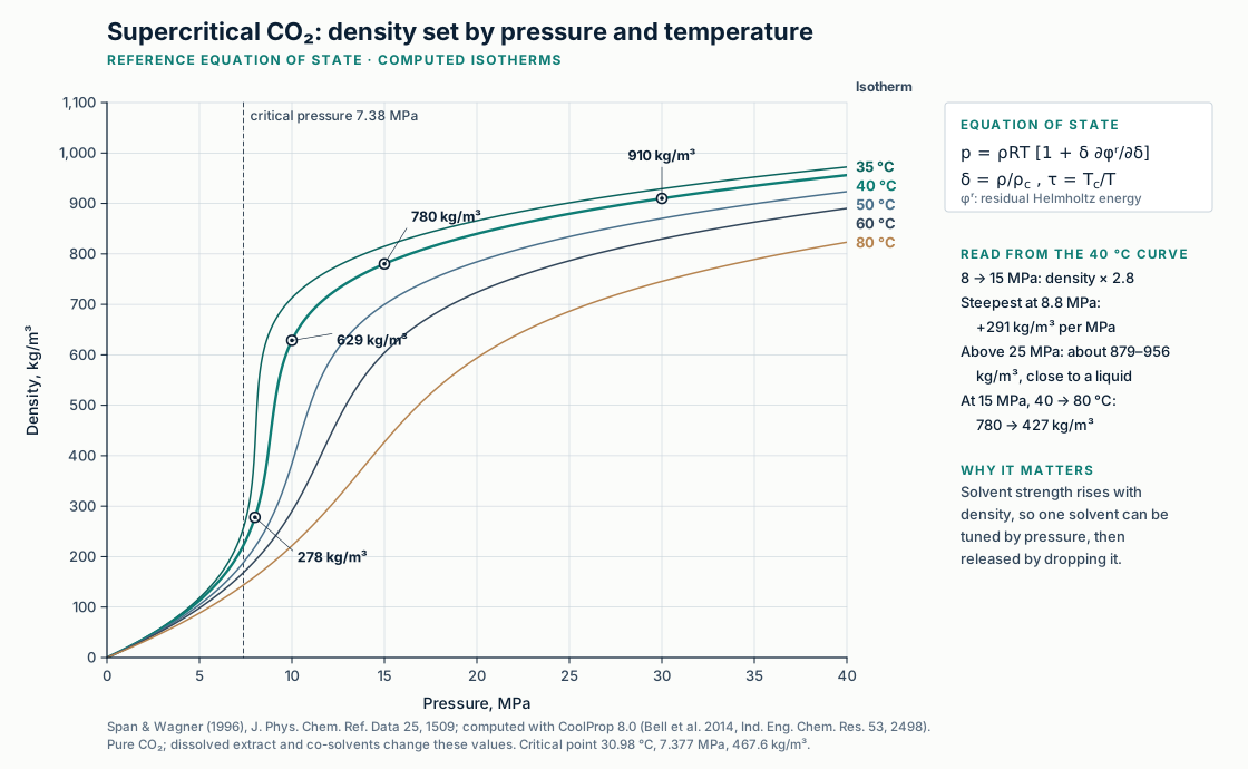
Planning a solvent-recovery, partitioning or crystallization step?
EUTECNIQ is in formation. We welcome conversations with partners about computing phase behavior before pilot work and measuring where the models disagree.