Design space and multi-objective optimization Published model reproduced Computed from published data Proposed capability

Optimizing an extraction means meeting every specification with stated confidence, then choosing by cost

One open-access botanical extraction study rebuilt from its published tables: response surfaces, desirability, a three-objective NSGA-II search and a probabilistic design space. Coefficients are the paper's; everything else is computed from its data.

16Box–Behnken runs, 3 factors at 3 levels (Gueffai et al. 2022, Table 1)

0.992R² of the TPC model; DPPH 0.973 (Table 2)

0.94highest probability that a new run meets TPC ≥ 32 and DPPH ≥ 62 inside the design sphere

5.9%of the design sphere reaches that probability at 0.80 or more

Status. EUTECNIQ has not run this experiment and has no laboratory data; the black cumin seed study is a published data set, and the page makes no health claim.

Academy fundamentals: Course 11, Multi-objective ingredient design

Reference molecules

Two reference molecules define the two responses: gallic acid for total phenolics and the DPPH radical for scavenging

The two reference molecules behind the two responsesComputed geometry

Assay references

Gallic acid

Formula: C₇H₆O₅
Molar mass: 170.12 g/mol
PubChem CID: 370
Role here: Calibration standard: total phenolic content is reported in mg gallic acid equivalent (GAE) per g

Drag or use the arrow keys to rotate. One gas-phase conformer each, not a crystal structure; MMFF94 is not parameterized for radicals, so the DPPH geometry is approximate.Structures: PubChem CIDs 370 and 2735032 (SMILES and formulas retrieved October 24, 2026); geometry: RDKit ETKDGv3 + MMFF94, one conformer (tools/mol3d.py). Assays as described by Gueffai et al. 2022, sections 2.5–2.6.

The published study

One open-access study publishes everything needed to rebuild its models: 16 runs, coded levels and both coefficient tables

The published extraction from seed to two assays, with its three factorsPublished study

Gueffai A, Gonzalez-Serrano DJ, Christodoulou MC, et al. Biomolecules. 2022;12(9):1311 (open access, CC BY 4.0), sections 2.3–2.6. Schematic, not to scale.

Text version of the experiment

Seeds bought at a local market in Mascara, Algeria (March 2022), milled and defatted with hexane.
Each run extracted 5 g of powder with 200 mL of ethanol–water in an ultrasonic bath at 110 W and 40 kHz.
Factors: ethanol 30, 60 and 90% (v/v); sonication temperature 25, 50 and 75 °C; sonication time 15, 30 and 45 min.
Responses: total phenolic content (TPC, Folin–Ciocalteu, mg gallic acid equivalent per g) and DPPH radical scavenging (% of the radical removed by a 2 mg/mL extract solution) In vitro.
Sixteen runs: 12 edge midpoints and 4 centre points, fitted with full second-order models.

The DPPH result is a chemical assay in a test tube. It says nothing about antioxidant effects in people.

Evidence key:Traditional useIn vitroAnimalHuman PKHuman RCTMeta-analysis of RCTs

Second-order polynomials in coded units put every coefficient on one scale

Second-order response-surface model (coded units)ŷ = β₀ + Σβ_ix_i + Σβ_iix_i² + ΣΣ_i<j β_ijx_ix_j

Coding maps each factor's low, middle and high levels to −1, 0 and +1, so a coefficient gives the change for a half-range step and the quadratic terms show curvature.

Coding of a factorx_i = X_i − X_i_,0ΔX_i e.g. x₁ = ethanol − 6030

The 16 Box–Behnken runs in factor space, colored by measured TPCPublished data

Drag to rotate, or use the buttons. The four centre points coincide at 60%, 50 °C, 30 min.

Show data (Table 1 of the paper)

Run	Ethanol (%)	Temperature (°C)	Time (min)	TPC (mg GAE/g)	DPPH (%)
1	60	25	45	28.4	65.1
2	30	25	30	25.7	44.8
3	60	75	15	21.8	35.5
4	60	50	30	35.1	70.5
5	30	50	45	24.3	39.4
6	90	25	30	24.5	44.5
7	30	50	15	24.3	36.8
8	60	50	30	35.6	68.0
9	60	75	45	21.1	44.5
10	60	50	30	35.2	69.1
11	60	50	30	35.1	69.0
12	60	25	15	22.2	41.5
13	90	75	30	19.2	45.4
14	90	50	45	22.6	64.0
15	30	75	30	20.4	35.0
16	90	50	15	19.3	38.8

Data: Gueffai et al. 2022, Table 1, copied exactly. Figure drawn by EUTECNIQ.

Curvature dominates both models; solid bars are significant at p < 0.05, and lack of fit is significant for bothPublished coefficients

A least-squares refit of the 16 published runs reproduces every Table 2 coefficient to within 0.005 and the same fit statistics; the page uses the published values. Significant lack of fit means predictions carry more error than R² suggests: the 95% prediction interval at the optimum is about ±2.3 mg GAE/g for TPC and ±9.9 points for DPPH.Gueffai et al. 2022, Table 2. Predicted R² and prediction intervals: EUTECNIQ computation from Table 1.

Text version: coefficient table and checks

Coded coefficient estimates and fit statistics, copied from Table 2 of the paper. x₁ ethanol, x₂ temperature, x₃ time.
Term	TPC coefficient	TPC p-value	DPPH coefficient	DPPH p-value
Intercept `β`₀	35.25	<0.0001 (model)	69.15	0.0005 (model)
`x`₁ ethanol	−1.14	0.0082	4.59	0.0118
`x`₂ temperature	−2.29	0.0002	−4.44	0.0136
`x`₃ time	1.10	0.0095	7.55	0.0011
`x`₁`x`₂	0.0000	1.0000	2.67	0.1914
`x`₁`x`₃	0.8250	0.0941	5.65	0.0209
`x`₂`x`₃	−1.72	0.0060	−3.65	0.0913
`x`₁²	−6.78	<0.0001	−14.31	0.0002
`x`₂²	−6.02	<0.0001	−12.41	0.0005
`x`₃²	−5.85	<0.0001	−10.09	0.0014
`R`² · adjusted `R`²	0.9924 · 0.9811		0.9728 · 0.9320
Coefficient of variation	3.20%		7.16%
Lack of fit (F, p)	23.34, 0.0140		24.00, 0.0134
Predicted `R`² (leave-one-out, EUTECNIQ computation)	0.883		0.580

The refit reproduces the table

A least-squares fit of the 16 published runs gives every Table 2 coefficient to within 0.005, and the same R², adjusted R², coefficient of variation and lack-of-fit F. The page uses the published coefficients.

EUTECNIQ computation

Lack of fit is significant for both models

The four centre points agree closely (pure error), and the residuals are larger than that agreement allows (p = 0.014 and 0.013). The quadratic surfaces miss some real structure, so predictions carry more error than R² suggests.

From Table 2

The DPPH model predicts new runs less well

Leaving each run out in turn and predicting it gives a predicted R² of 0.883 for TPC and 0.580 for DPPH. The 95% prediction interval at the optimum is about ±2.3 mg GAE/g for TPC and ±9.9 points for DPPH.

EUTECNIQ computation

Explanation, details and sources

Gueffai and co-authors optimized ultrasound-assisted extraction of phenolics from defatted black cumin seed (Nigella sativa L.) with a three-factor Box–Behnken design: runs at the edge midpoints of the experimental cube plus repeated centre points.

Two reporting errors in the paper do not affect these models: the text's Equation (2) lists Table 2's F-values as DPPH coefficients, and the text swaps two HPLC concentrations relative to Table 4. The refit confirms Table 2.

Response surfaces and desirability

Both responses peak near 60% ethanol and 45 °C, and the desirability optimum reproduces the authors' reported conditions

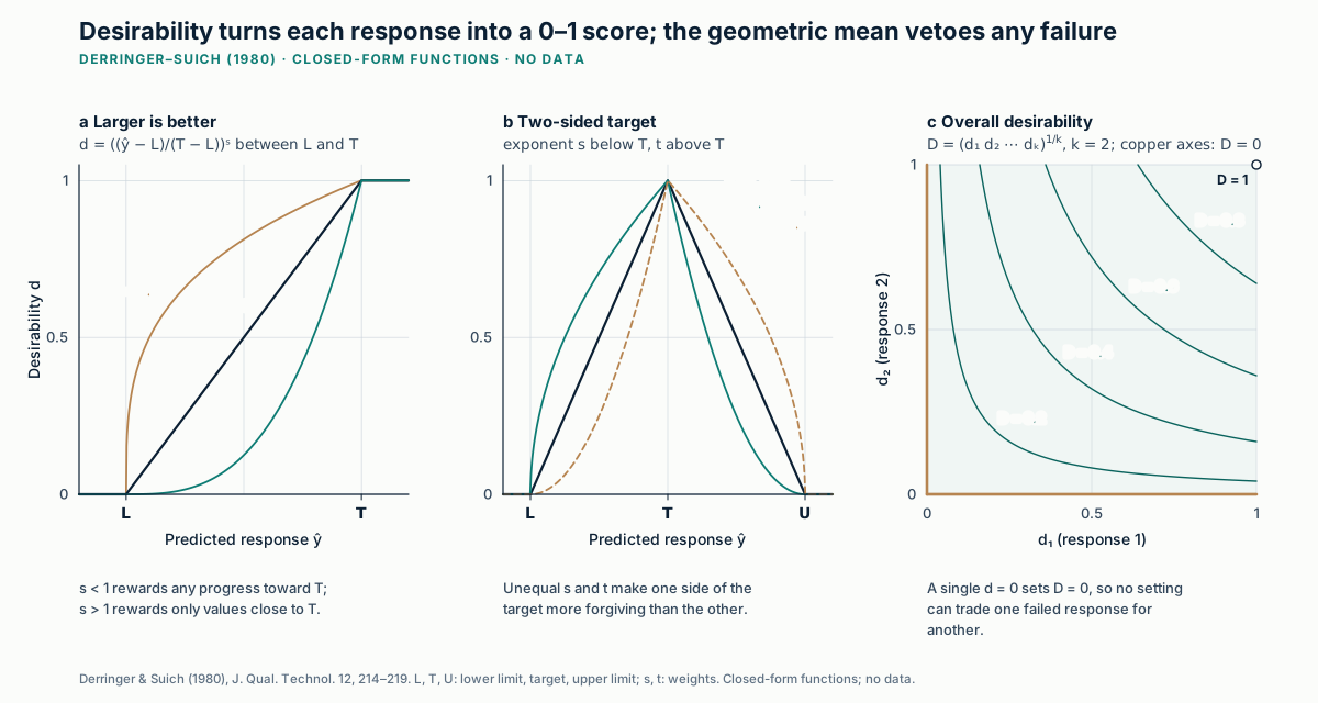
Derringer–Suich: larger is better (smaller is better mirrors it)d = 0 for ŷ ≤ L; d = (ŷ − LT − L)^s; d = 1 for ŷ ≥ T

Target is best · overall desirability of k responsesd = (ŷ − LT − L)^s below T, (U − ŷU − T)^t above
D = (d₁ d₂ ⋯ d_k)^1/k

Sonication time (third factor; the surface is this slice) Probe point: ethanol Probe point: temperature Specification: minimum TPC Specification: minimum DPPH Stay inside the design sphere (radius √2 in coded units), where the runs were made

Desirability settings (limits, targets, exponents)

TPC (mg GAE/g) Goal Lower limit L Target T Upper limit U (target or minimize) Exponent s (weight)

DPPH (% scavenged) Goal Lower limit L Target T Upper limit U (target or minimize) Exponent s (weight)

TPC at the probe

95% prediction interval

DPPH at the probe

95% prediction interval

D at the probe

Slice meeting both specifications

Optimum: ethanol

temperature

time

Maximum D

TPC at the optimum

DPPH at the optimum

Desirability over ethanol and temperature at the selected timeReproduced model

Amber marks conditions whose predicted TPC and DPPH both meet the specifications. The ring marks the best D in this slice; the blue dot is the probe point.

Show data (predictions on a 7 × 7 grid of this slice)

Ethanol (%)	25 °C	33.3 °C	41.7 °C	50 °C	58.3 °C	66.7 °C	75 °C
The table fills in when the page's scripts run; Table 2 above gives the model needed to compute any value.

Reproduced from Gueffai et al. 2022 (Table 2 coefficients; coding ±1 = 30–90% ethanol, 25–75 °C, 15–45 min). EUTECNIQ has not run this experiment. Corners of the cube lie outside the design sphere and are extrapolations.Derringer G, Suich R. J Qual Technol. 1980;12(4):214–219; NIST/SEMATECH e-Handbook of Statistical Methods, section 5.5.3.2.2.

Method, assumptions and limits

What it calculates: Predicted TPC and DPPH from the published coded models at any ethanol, temperature and time; Derringer–Suich individual and overall desirability; the slice of conditions meeting both specifications; the global desirability optimum; 95% prediction intervals at the probe point.
Equations: Models as in the table above. d_i as defined by Derringer and Suich (maximize, minimize or target, with exponents s and t; the page uses t = s); D = (d₁d₂)^1/2. Prediction interval ±t_{0.975, 6} s_e √(1 + zᵀ(XᵀX)⁻¹z), with t_{0.975, 6} = 2.447 and residual standard deviations s_e = 0.830 (TPC) and 3.634 (DPPH) from the refit of Table 1.
Variables and units: Coded x₁ = (ethanol − 60)/30, x₂ = (temperature − 50)/25, x₃ = (time − 30)/15; TPC in mg GAE/g; DPPH in % scavenged.
Optimum search: A 41 × 41 × 41 grid over the coded cube, then a pattern search with fixed pseudo-random directions to a step of 10⁻⁷, inside the design sphere when that option is on. The slice fraction counts a 61 × 61 grid.
Assumptions: The quadratic models hold within the design region; errors are independent and normal with constant variance; one lot of seed and one bath.
Valid range: 30–90% ethanol, 25–75 °C, 15–45 min. Inside the sphere of radius √2 the models interpolate between runs; at the cube's corners they extrapolate. Limits are reordered if a lower limit exceeds a target, and a warning appears.
What it does not establish: Performance at other scales, other seed lots or other equipment; any health effect; a validated design space. Significant lack of fit means the surfaces are approximations.
References: Gueffai et al. 2022; Box and Behnken 1960; Derringer and Suich 1980; NIST/SEMATECH e-Handbook 5.5.3.2.2.
Verification: An independent Python reference (numpy, scipy) recomputes the predictions, prediction intervals, slice fractions and optima, including the authors' reported optimum, in tests/numerics/ref/insights-design-space-optimization.py.

Explanation, details and sources

Desirability turns each response into a score between 0 (unacceptable) and 1 (fully satisfactory) and combines them with a geometric mean, so a single unacceptable response sets the total to zero. With the scores spanning the observed ranges, the optimum falls at 59.2% ethanol, 44.7 °C and 32.5 min. The authors report 59.18%, 44.68 °C and 32.51 min.

Three panels. Left: a larger-is-better desirability rises from 0 at the lower limit L to 1 at the target T, concave for weight 0.3, straight for 1 and convex for 3. Middle: a two-sided target desirability peaks at the target and falls to 0 at the lower and upper limits, with weights shaping each side. Right: lines of equal overall desirability, the geometric mean of two individual desirabilities, which is 0 whenever either is 0. Closed-form functions from Derringer and Suich (1980); no data. — Derringer G, Suich R. J Qual Technol 1980;12:214–219. Closed-form functions; no data. Generated illustration, EUTECNIQ. Full-size SVG

Three objectives and NSGA-II

A third objective, sonication time, turns one optimum into a front of trade-offs that NSGA-II maps in about 60 generations

Each NSGA-II generation ranks conditions into non-dominated fronts and keeps the best-ranked, best-spread halfSchematic of the published algorithm

Condition a dominates b when a is no worse in every objective and strictly better in at least one; the non-dominated set is the Pareto front.Deb K, Pratap A, Agarwal S, Meyarivan T. IEEE Trans Evol Comput. 2002;6(2):182–197. Operators and settings as in pymoo 0.6 (Blank and Deb, IEEE Access 2020).

Text version of the NSGA-II steps

Definitions

Condition a dominates b when a is no worse in every objective and strictly better in at least one. The non-dominated set is the Pareto front.

Start. Draw a population of random conditions inside the cube.
Make offspring. Pick parents by binary tournament, recombine them with simulated binary crossover and perturb them with polynomial mutation.
Sort. Merge parents and offspring; rank them into successive non-dominated fronts (fast non-dominated sorting).
Spread. Within a front, prefer points with a larger crowding distance, the size of the gap to their neighbours along each objective.
Survive. Keep the best-ranked half and repeat. Conditions outside the design sphere lose to any condition inside it (constrained domination).

Deb K, Pratap A, Agarwal S, Meyarivan T. IEEE Trans Evol Comput. 2002;6(2):182–197. Operators and settings as in pymoo 0.6 (Blank and Deb, IEEE Access 2020).

Measuring a front

Hypervolume of a front P (objectives normalized, minimized)HV(P) = vol( ∪_p∈P [p₁, 1] × [p₂, 1] × [p₃, 1] )

How the hypervolume is scaled

Objectives are scaled from an ideal value (0) to a reference value (1): TPC 36 to 20 mg GAE/g, DPPH 72 to 35%, time 15 to 45 min. The hypervolume is the fraction of that unit box the front dominates; larger is better.

Zitzler E, Thiele L. IEEE Trans Evol Comput. 1999;3(4):257–271; slicing algorithm: While L et al. IEEE Trans Evol Comput. 2006;10(1):29–38.

Population size Generations Random seed Constrain the search to the design sphere

Generation

Points on the front

Hypervolume

pymoo, same budget (60 × 60, seed 1)

Dominated pairs within the front

Highest TPC on the front

Highest DPPH on the front

Shortest time meeting TPC ≥ 32 and DPPH ≥ 62

A large pymoo run (population 200, 300 generations) reaches a hypervolume of 0.785; that is close to the best this problem allows.

Population in objective space: non-dominated front and the restOptimization of a reproduced model

Show data (current front, sorted by time)

Time (min)	Ethanol (%)	Temperature (°C)	TPC (mg GAE/g)	DPPH (%)
The table fills in when the optimizer runs.

Objectives evaluated with the published models (Gueffai et al. 2022). The reference front (blue) is a pymoo 0.6.2 NSGA-II run with population 60, 60 generations and seed 1, computed offline. Points beyond about 37 min never reach the front, because in the models longer sonication lowers both responses. Points outside the plotted ranges (early generations) are not drawn.

Method, assumptions and limits

What it calculates: A three-objective Pareto front for the published models (maximize TPC, maximize DPPH, minimize sonication time), its hypervolume, and checks that its points are mutually non-dominated.
Algorithm: NSGA-II with constrained domination (feasible before infeasible; infeasible ranked by violation of xᵀx ≤ 2); binary tournament on domination and crowding distance; simulated binary crossover (η_c = 15, probability 0.9 per mating, 0.5 per variable); polynomial mutation (η_m = 20, probability 1/3 per variable); elitist survival on rank, then crowding distance.
Determinism: A seeded 32-bit generator (mulberry32) drives every random choice, so the same seed gives the same run in any browser. Play animates one generation at a time; with reduced motion it jumps to the end.
Hypervolume: Exact, by sweeping the time objective and summing two-dimensional dominated areas between successive time levels (hypervolume by slicing objectives).
Assumptions: Objectives are mean model predictions; uncertainty is treated in the next section. Time stands in for cost because power was constant.
What it does not establish: That front points meet specifications in practice. A point chosen at a specification limit has, at best, an even chance of meeting it.
References: Deb et al. 2002; Blank and Deb 2020; Zitzler and Thiele 1999; While et al. 2006.
Verification: The Python reference runs pymoo's NSGA2 with the same objectives and constraint and its hypervolume indicator. The page's run must come within 3% of pymoo's hypervolume for the same budget, and its front must contain no dominated pair. The same hypervolume routine applied to pymoo's stored front returns pymoo's own value to 10⁻⁶.

The 60 Pareto-optimal conditions on four axes: drag along an axis to keep only the conditions you would acceptComputed from published data

Each line is one condition on the pymoo reference front (population 60, 60 generations, seed 1); the selection text lists ethanol, temperature and time. P(both specs) is the posterior predictive probability that a new run meets TPC ≥ 32 mg GAE/g and DPPH ≥ 62%, computed as in the next section.Front: archived pymoo 0.6.2 run on the published models (Gueffai et al. 2022). Probabilities: bivariate t posterior predictive (Peterson 2004), SciPy multivariate_t.cdf; script src/modules/comp_ds/compute/make_data.py.

Data table: the 60 front points

The 60 points of the NSGA-II reference front (pymoo 0.6.2), sorted by sonication time, with the probability of meeting TPC ≥ 32 and DPPH ≥ 62
Ethanol (% v/v)	Temperature (°C)	Time (min)	TPC (mg GAE/g)	DPPH (%)	P(both)
60.9	54.5	15.0	27.94	50.94	0.00
56.5	49.1	15.0	28.45	51.46	0.00
60.9	47.2	15.4	28.56	52.13	0.00
57.8	51.6	15.5	28.78	52.33	0.00
62.7	46.4	15.8	28.70	52.60	0.00
61.1	49.4	15.8	28.89	52.91	0.00
53.4	49.2	15.8	29.07	52.46	0.00
61.0	47.2	16.1	29.11	53.33	0.00
51.4	48.4	16.2	29.29	52.72	0.00
53.4	48.4	16.4	29.52	53.43	0.00
57.2	47.2	16.6	29.71	54.24	0.00
62.2	47.2	16.9	29.64	54.67	0.00
61.1	47.1	17.2	30.02	55.37	0.00
61.3	46.9	17.4	30.09	55.56	0.00
60.9	47.2	17.5	30.22	55.80	0.00
60.9	47.2	17.7	30.41	56.23	0.00
57.1	46.4	17.9	30.66	56.32	0.00
61.0	45.9	17.9	30.48	56.41	0.00
60.0	47.2	18.5	30.98	57.42	0.00
57.4	47.2	18.9	31.36	57.92	0.00
58.9	47.2	19.2	31.51	58.48	0.01
60.8	47.2	19.3	31.49	58.71	0.01
61.2	46.5	19.6	31.66	59.14	0.01
55.8	48.6	19.8	31.95	59.08	0.02
57.4	44.2	19.9	31.92	59.22	0.02
55.1	48.6	20.1	32.14	59.41	0.04
58.8	48.6	20.2	32.13	59.90	0.05
57.5	47.2	20.4	32.32	60.17	0.08
57.5	47.4	20.6	32.40	60.35	0.10
56.5	47.2	21.1	32.72	60.97	0.19
60.9	47.2	21.1	32.57	61.29	0.18
60.9	47.2	21.5	32.74	61.70	0.25
59.5	47.4	21.6	32.91	61.89	0.30
58.5	46.0	23.3	33.76	63.82	0.58
64.2	47.2	23.8	33.54	64.42	0.60
53.2	46.0	23.9	33.90	63.36	0.56
53.3	46.0	24.2	34.05	63.75	0.60
57.7	48.5	24.4	34.16	64.78	0.68
57.4	48.6	26.1	34.73	66.31	0.79
61.0	47.2	26.9	34.86	67.49	0.85
61.1	47.1	27.2	34.94	67.78	0.86
54.9	45.5	27.4	35.06	66.86	0.82
61.1	45.6	28.2	35.15	68.49	0.89
61.1	46.1	28.6	35.23	68.81	0.90
57.0	46.1	28.6	35.33	68.18	0.88
59.2	47.2	29.3	35.39	69.00	0.90
56.5	43.8	30.1	35.50	68.90	0.90
61.4	44.9	30.7	35.46	70.06	0.93
61.2	46.1	31.6	35.49	70.45	0.93
56.5	44.5	31.7	35.59	69.62	0.92
57.9	44.5	31.9	35.59	70.02	0.93
65.0	48.6	32.3	35.04	70.80	0.93
60.0	46.5	32.8	35.49	70.70	0.94
67.1	44.5	34.0	34.85	71.54	0.94
60.8	47.2	34.9	35.20	71.17	0.94
66.8	44.7	35.7	34.64	71.91	0.94
67.1	44.5	36.2	34.51	71.95	0.94
67.2	44.4	36.7	34.39	71.99	0.93
66.9	44.4	37.3	34.26	72.00	0.93
67.2	44.4	37.3	34.22	72.00	0.92

Along the front, trimming sonication from about 32 to 21 minutes drops the chance of meeting both specifications from 0.93 to 0.18.

Explanation, details and sources

A Pareto search postpones the trade-off choice that desirability fixes in advance: it returns every condition that cannot improve one objective without losing another. Objectives: maximum TPC, maximum DPPH, minimum sonication time (a stated proxy for energy use and throughput, since the bath ran at a constant 110 W).

Probabilistic design space

Accounting for model uncertainty shrinks the region that meets both specifications, and the cheapest conditions on the mean front often fail

Bayesian design space (Peterson)DS = { x : Pr( TPC ≥ a and DPPH ≥ b | x, data ) ≥ R }

Posterior predictive for two responses, noninformative priory | x ~ t_ν( B̂ᵀz, (1 + zᵀ(XᵀX)⁻¹z) S/ν ), ν = n − p − r + 1 = 5

Sonication time (slice) Specification: minimum TPC Specification: minimum DPPH Required reliability R

Probability at the authors' optimum (59.1%, 44.6 °C, 32.5 min)

Slice where mean predictions meet both

Slice with probability ≥ R

Highest probability in this slice

at ethanol, temperature

Posterior probability of meeting both specifications over ethanol and temperatureComputed from published data

Height and color show the probability. Amber marks conditions that meet both specifications with at least the required reliability.

Computed by EUTECNIQ from Table 1 of Gueffai et al. 2022 with 4,000 seeded Monte Carlo draws; Monte Carlo error is about ±0.01. EUTECNIQ has not run this experiment.Peterson JJ. J Qual Technol. 2004;36(2):139–153; Peterson JJ. J Biopharm Stat. 2008;18(5):959–975; ICH Q8(R2), Step 4, August 2009, glossary.

Method, assumptions and limits

What it calculates: For each condition in the slice, the probability that a new run would give TPC and DPPH at or above the specifications, given the 16 published runs; the share of the slice meeting the specifications on mean predictions and with probability of at least R.
Model: Both responses share the quadratic design matrix X (16 × 10). Under the noninformative prior p(B, Σ) ∝ |Σ|^−3/2, the predictive distribution of a new pair of responses is bivariate t with ν = 16 − 10 − 2 + 1 = 5 degrees of freedom, location B̂ᵀz(x) and scale (1 + h)S/ν, where S is the residual cross-product matrix and h the leverage. The residual correlation between TPC and DPPH is −0.80 and is kept.
Monte Carlo: 4,000 draws of (z₁, z₂, w) with z standard normal and w ~ χ²₅, fixed seed, reused at every grid point (31 × 31) so the surface is smooth.
Assumptions: The quadratic model is correct; errors are normal, independent and of constant variance; no prior information. Significant lack of fit means the model is not fully correct, so these probabilities are optimistic in that respect.
What it does not establish: A design space in the regulatory sense. ICH Q8(R2) requires demonstration, which means confirmation runs at the chosen conditions and, for scale-up, evidence that the region holds at production scale. Dietary supplements have no design-space filing.
References: Peterson 2004 and 2008 (approach; full texts not accessed, abstracts verified); van de Berg et al. 2021 (a Monte Carlo probabilistic design space in a QbD study); ICH Q8(R2).
Verification: The Python reference evaluates the same probabilities with 10⁶ independent draws and checks the closed form against hierarchical sampling (inverse-Wishart covariance, matrix-normal coefficients); the three agree to within 0.001 at the authors' optimum.

Required probability R0.80

Grid points with P ≥ R117

Share of the design sphere5.9%

The design space as a volume: every grid condition inside the design sphere that meets both specifications with probability ≥ RComputed from published data

13 × 13 × 13 grid over the coded cube, kept inside the design sphere (1,989 points); specifications TPC ≥ 32 mg GAE/g and DPPH ≥ 62%. The ring marks the authors' reported optimum (P = 0.93). EUTECNIQ has not run this experiment.Peterson 2004; probabilities with SciPy multivariate_t.cdf from the refit of Gueffai et al. 2022, Table 1 (src/modules/comp_ds/compute/make_data.py).

Data table: share of the design sphere for four values of R

Share of the design sphere where the probability of meeting both specifications reaches R (1989 grid points)
R	Share of the design sphere
0.50	13.1%
0.80	5.9%
0.90	2.1%
0.95	0.0%

At R = 0.80 the design space is 117 of 1,989 grid points (5.9% of the design sphere), and no condition reaches 0.95.

The shortest time that meets a specification on the mean meets it with well under even odds

Cutting sonication to the mean-prediction minimum drops the chance of meeting both specifications to 0.10–0.45Computed from published data

For each specification: the shortest time whose mean predictions meet both limits, and the chance a new run there meets them.Computed by EUTECNIQ from the published models and data (grid search and SLSQP inside the design sphere; 10⁶ predictive draws per probability). Script: src/modules/designspace/compute/tradeoffs.py.

Show data

Specification (TPC, DPPH)	Shortest time on the mean	At ethanol, temperature	Probability of meeting both there	Probability at the authors' optimum (32.5 min)
≥ 30 mg GAE/g, ≥ 60%	20.2 min	60.7%, 48.0 °C	0.45	0.97
≥ 32 mg GAE/g, ≥ 62%	21.7 min	61.3%, 47.7 °C	0.29	0.93
≥ 34 mg GAE/g, ≥ 65%	24.2 min	61.2%, 47.0 °C	0.10	0.77
≥ 35 mg GAE/g, ≥ 68%	27.5 min	61.3%, 46.1 °C	0.10	0.41

Computed by EUTECNIQ from the published models and data (grid search and SLSQP inside the design sphere; 10⁶ predictive draws per probability). Script: src/modules/designspace/compute/tradeoffs.py.

Explanation, details and sources

ICH Q8(R2) defines a design space as the combination of input variables and process parameters "that have been demonstrated to provide assurance of quality." Peterson proposed measuring that assurance as the posterior predictive probability that every response meets its specification, and accepting conditions where it exceeds a chosen reliability.

Limits and use

Models of one seed lot in one laboratory bath guide the next experiments but establish nothing about health or plant scale

DPPH radical scavenging in a test tube≠an antioxidant effect in people
High R² on the design runs≠good prediction of new runs (predicted R² 0.58 for DPPH)
Desirability optimum≠design space
Model probability≠demonstrated assurance (confirmation runs are needed)
Laboratory ultrasonic bath≠a plant-scale extractor

The proposed workflow has five stages; this page shows the middle three on published dataProposed workflow

EUTECNIQ proposal. Screening and confirmation require new experiments on qualified material.

Text version of the proposed workflow

ScreenFractional factorial or Plackett–Burman runs rank many candidate factors
ModelBox–Behnken or central composite runs fit second-order models; lack of fit and predicted R² reported
Trade offDesirability for a fixed priority; NSGA-II with cost, solvent or time for an open choice
Quantify riskPosterior probability of meeting every specification; region chosen at a stated reliability
Confirm and scaleNew runs inside the region; scale-dependent parameters checked at pilot scale before transfer

Explanation, details and sources

The methods transfer to any botanical process; the numbers do not. A real program would repeat the design on qualified material, confirm the region with new runs and check it at pilot scale.

Related pages: QbD basics and a simulated response-surface example on process engineering and scale-up; QTPP, CQAs, CPPs and control strategy on QbD and control strategy; Gaussian-process and Bayesian optimization on botanical intelligence.

Plan a designed experiment on your material

Partners can describe a botanical process and its specifications; EUTECNIQ would propose a design, the analyses it supports and what it would not establish.

Contact EUTECNIQ QbD and control strategy